
Spatial Data and Mapping


Grayson White

Stat 241
Week 5 | Fall 2026

Math / Stats / CS Hike!!!

This year’s annual Math/Stats/CS picnic-hike will take place on Saturday, October 10th, from approximately 9:00am (leave Reed) until approximately 2:00pm (return to Reed). The location of the hike is Tryon Creek State Natural Area (approx 7.5 miles from Reed).

A boxed lunch will be provided. Hiking trails are available but don’t feel like you have to hike - there will be games and other activities available at the picnic tables.

Please use this link to sign-up and order a lunch which the departments will cover.

Deadline to sign up is Thursday at Noon - 10/01.

Week 5 Goals

Mon Lecture

  • Joining multiple data frames
  • “Tidy” data
  • Reshaping data frames

Wed Lecture

  • Introduction to spatial data
    • point data
    • polygon data
  • Static and interactive maps with point and polygon data
    • base layers (almost as good as merino)
    • coordinate reference systems / projections
    • popups and additional context
    • static graphs with sf and ggplot2
    • interactive graphs with leaflet

Spatial Data

  • Data that is linked to the physical world.

  • Example: Crash data in Portland from Problem Sets 2 and 3!

  • Visualizing these data on a map (or map-like graph) is a great way to add useful context!

Focus on creating the following types of maps:

  • Point maps

  • Choropleth maps

  • Cartograms

  • Hexbin maps (cartogram heatmaps)

  • Interactive maps

  • Raster maps (Wednesday)

Spatial Data Example: Cholera Outbreak in 1854

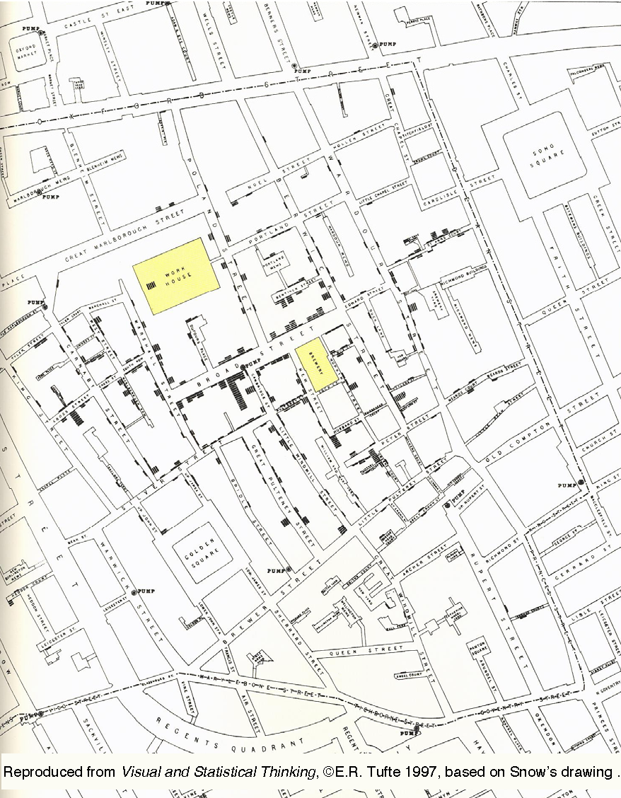
The most famous early analysis of geospatial data was done by physician John Snow in 1854.

Cholera outbreaks were common in 19th century London

  • believed to be an airborne disease caused by breathing foul air

Outbreak in 1854: over 600 deaths in Soho, London

  • John Snow collects data, thinks contaminated water is the cause

  • At the time water was provided by competing private firms from water pumps

  • Snow recorded locations of (i) deaths and (ii) water pumps

A simple visual model (Tobler 1994):

This figure:

  • Red Dots: Cholera cases

  • Blue Triangles: Pumps

  • Blue Lines: Closest pump is contained in each section


Q: What pattern do you notice?

Q: What are some possible explanations for the “outliers”? (deaths that don’t match up with the pattern)
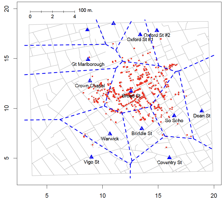
Conclusion: Visualizing spatial data can help us see key patterns

Static Maps
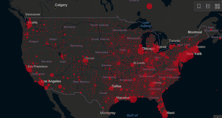
Source: JHU

Choropleth Maps

Source: The Guardian
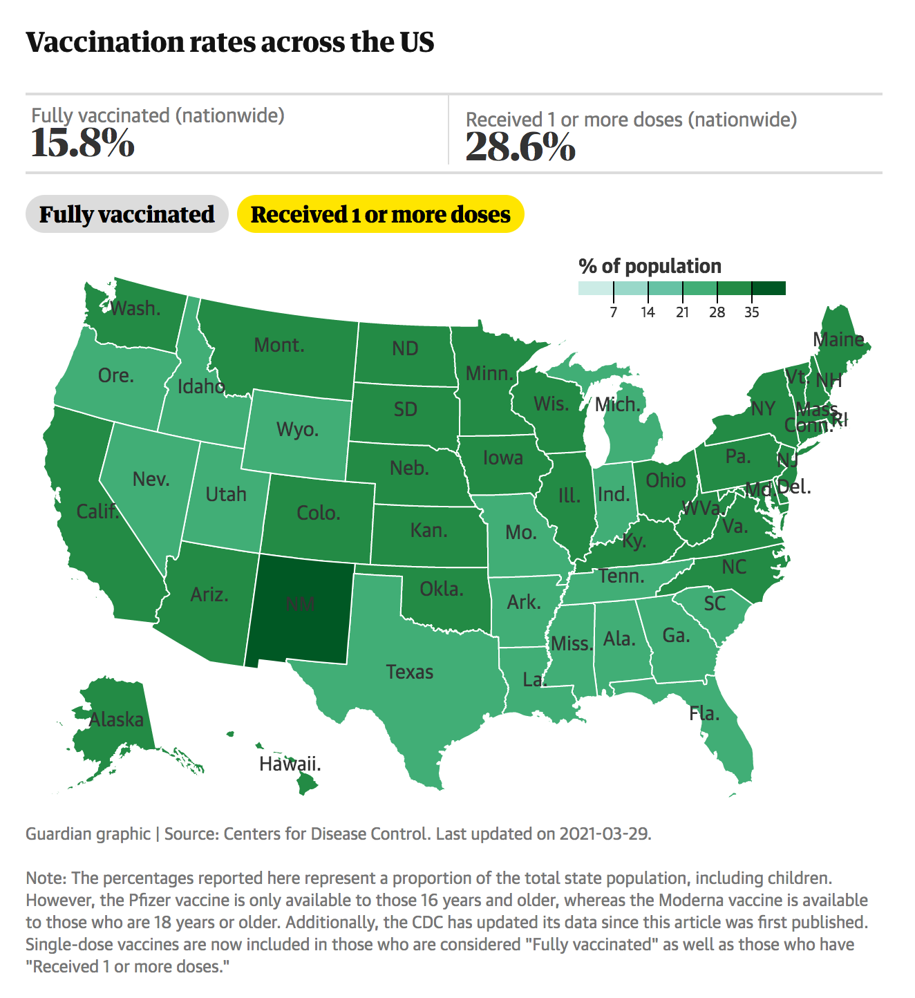
Choropleth Maps
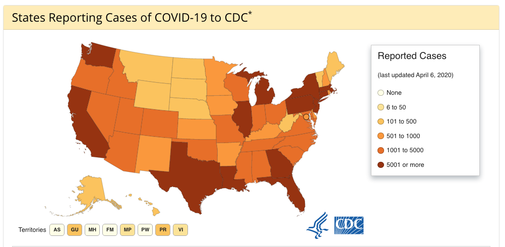
Source: CDC

Choropleth Maps
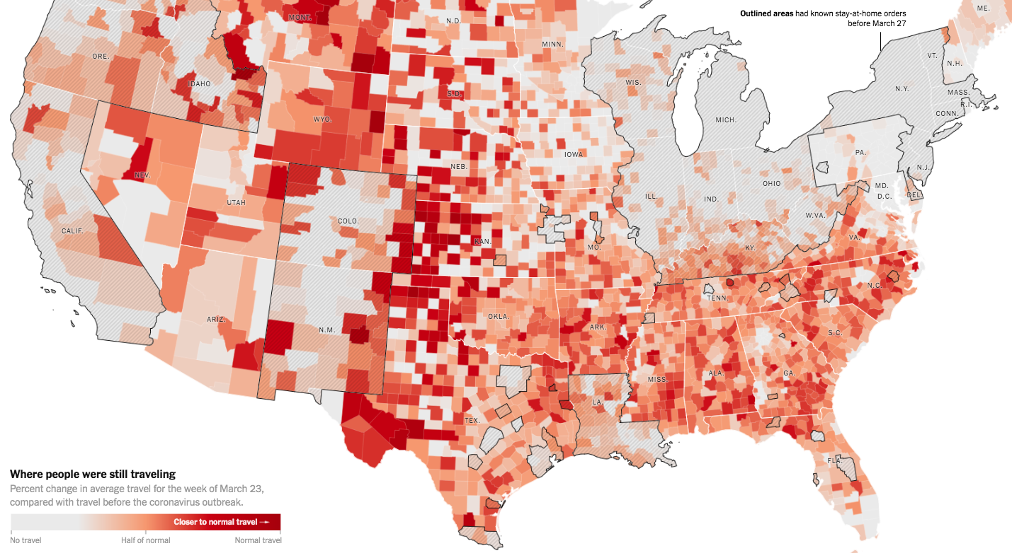
Source: NYtimes.com

Choropleth Maps
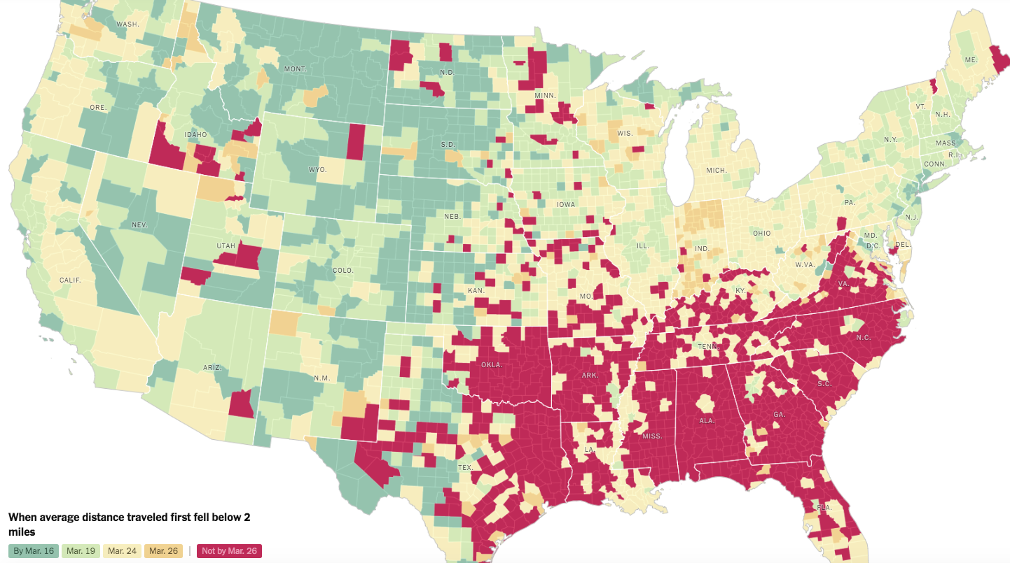
Source: NYtimes.com

Cartogram
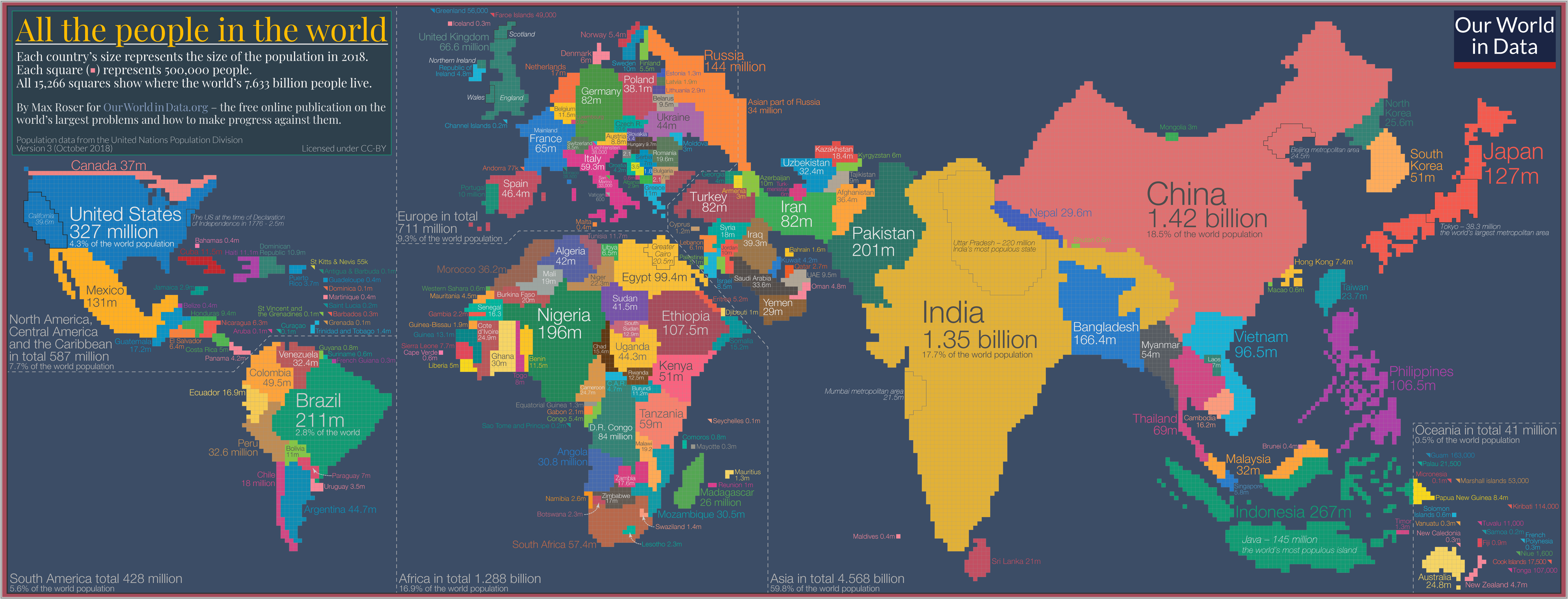
Source: Our World in Data

“Hex”bin Maps
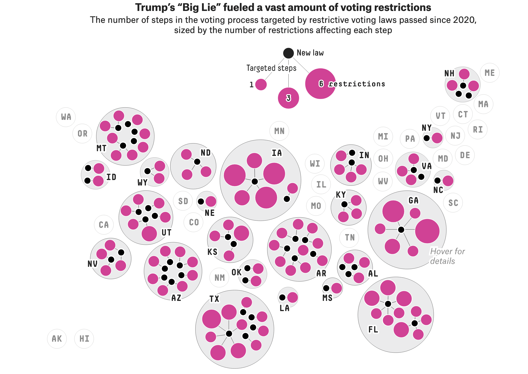
Source: FiveThirtyEight

Interactive Maps
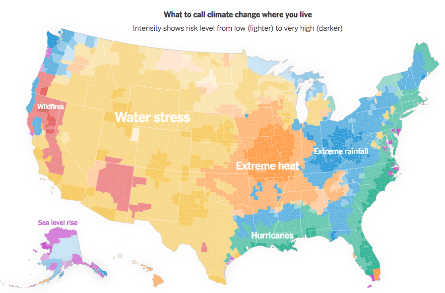
Source: NYTimes

Spatial Data Structures

  • Often stored in special data structures
    • Ex: Shapefile(s)
    • Consist of geometric objects like points, lines, and polygons
  • Visualizing Spatial Data
    • Need to draw the map
    • Add metadata on top of the map
      • Color in regions
      • Dots

Let’s begin with data from the forested R package

library(forested)
data(forested)
glimpse(forested)
Rows: 7,107
Columns: 20
$ forested         <fct> Yes, Yes, No, Yes, Yes, Yes, Yes, Yes, Yes, Yes, Yes,…
$ year             <dbl> 2005, 2005, 2005, 2005, 2005, 2005, 2005, 2005, 2005,…
$ elevation        <dbl> 881, 113, 164, 299, 806, 736, 636, 224, 52, 2240, 104…
$ eastness         <dbl> 90, -25, -84, 93, 47, -27, -48, -65, -62, -67, 96, -4…
$ northness        <dbl> 43, 96, 53, 34, -88, -96, 87, -75, 78, -74, -26, 86, …
$ roughness        <dbl> 63, 30, 13, 6, 35, 53, 3, 9, 42, 99, 51, 190, 95, 212…
$ tree_no_tree     <fct> Tree, Tree, Tree, No tree, Tree, Tree, No tree, Tree,…
$ dew_temp         <dbl> 0.04, 6.40, 6.06, 4.43, 1.06, 1.35, 1.42, 6.39, 6.50,…
$ precip_annual    <dbl> 466, 1710, 1297, 2545, 609, 539, 702, 1195, 1312, 103…
$ temp_annual_mean <dbl> 6.42, 10.64, 10.07, 9.86, 7.72, 7.89, 7.61, 10.45, 10…
$ temp_annual_min  <dbl> -8.32, 1.40, 0.19, -1.20, -5.98, -6.00, -5.76, 1.11, …
$ temp_annual_max  <dbl> 12.91, 15.84, 14.42, 15.78, 13.84, 14.66, 14.23, 15.3…
$ temp_january_min <dbl> -0.08, 5.44, 5.72, 3.95, 1.60, 1.12, 0.99, 5.54, 6.20…
$ vapor_min        <dbl> 78, 34, 49, 67, 114, 67, 67, 31, 60, 79, 172, 162, 70…
$ vapor_max        <dbl> 1194, 938, 754, 1164, 1254, 1331, 1275, 944, 892, 549…
$ canopy_cover     <dbl> 50, 79, 47, 42, 59, 36, 14, 27, 82, 12, 74, 66, 83, 6…
$ lon              <dbl> -118.6865, -123.0825, -122.3468, -121.9144, -117.8841…
$ lat              <dbl> 48.69537, 47.07991, 48.77132, 45.80776, 48.07396, 48.…
$ land_type        <fct> Tree, Tree, Tree, Tree, Tree, Tree, Non-tree vegetati…
$ county           <fct> Ferry, Thurston, Whatcom, Skamania, Stevens, Stevens,…

What we’ve done so far:

ggplot(forested, aes(x = lon, 
                     y = lat,
                     color = forested)) + 
  geom_point(size = 0.5) + 
  scale_color_manual(
    values = c("forestgreen", "goldenrod3")
    )

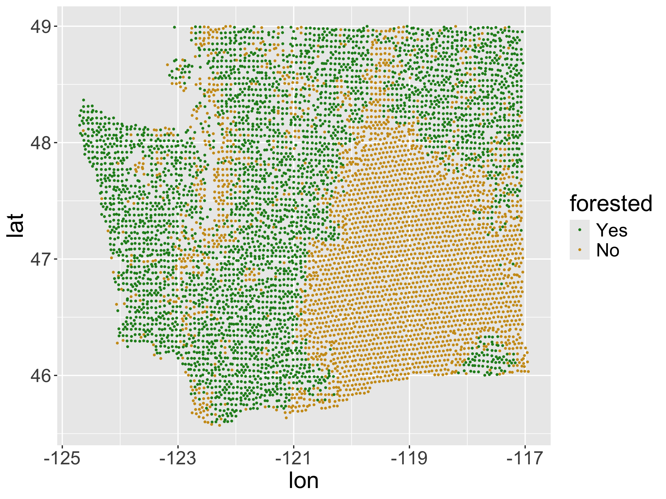
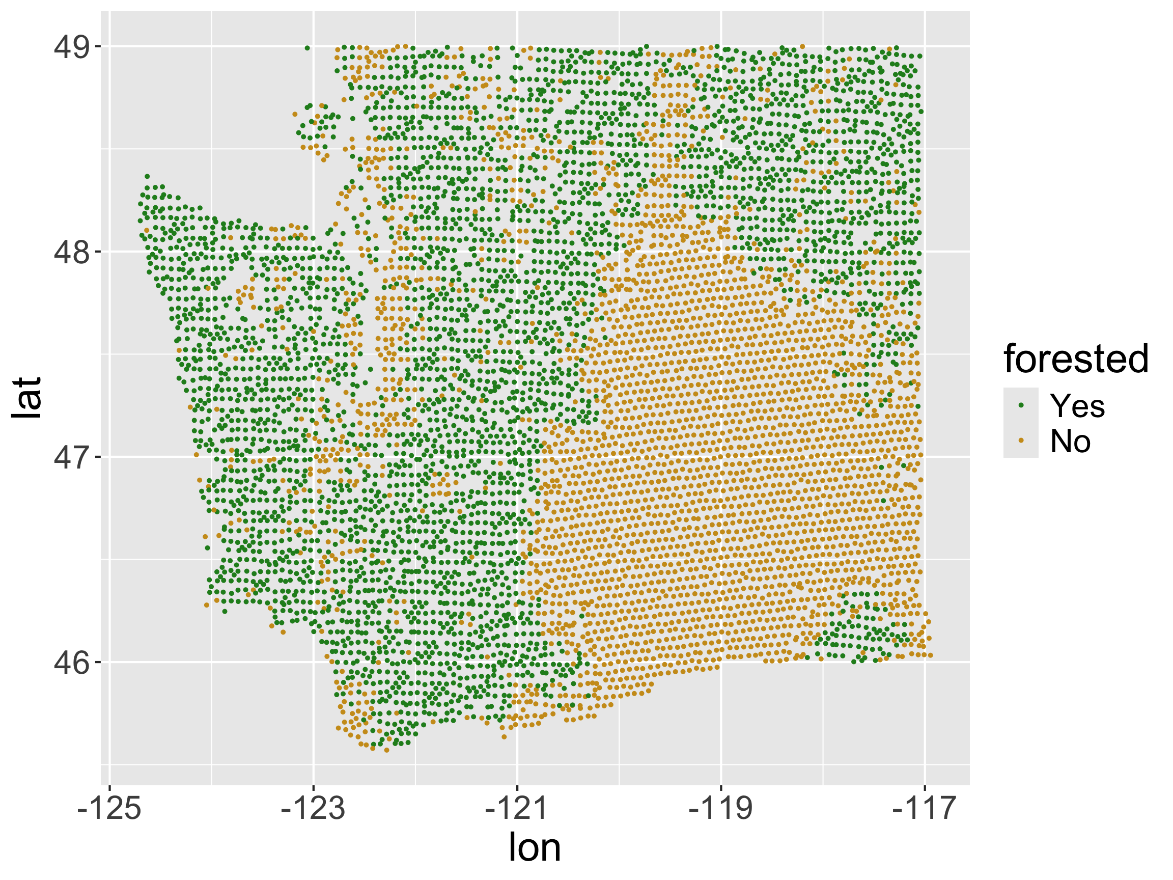
  • x-axis: longitude, y-axis: latitude
  • No projection
  • No base layer
  • Let’s improve it!

Projections

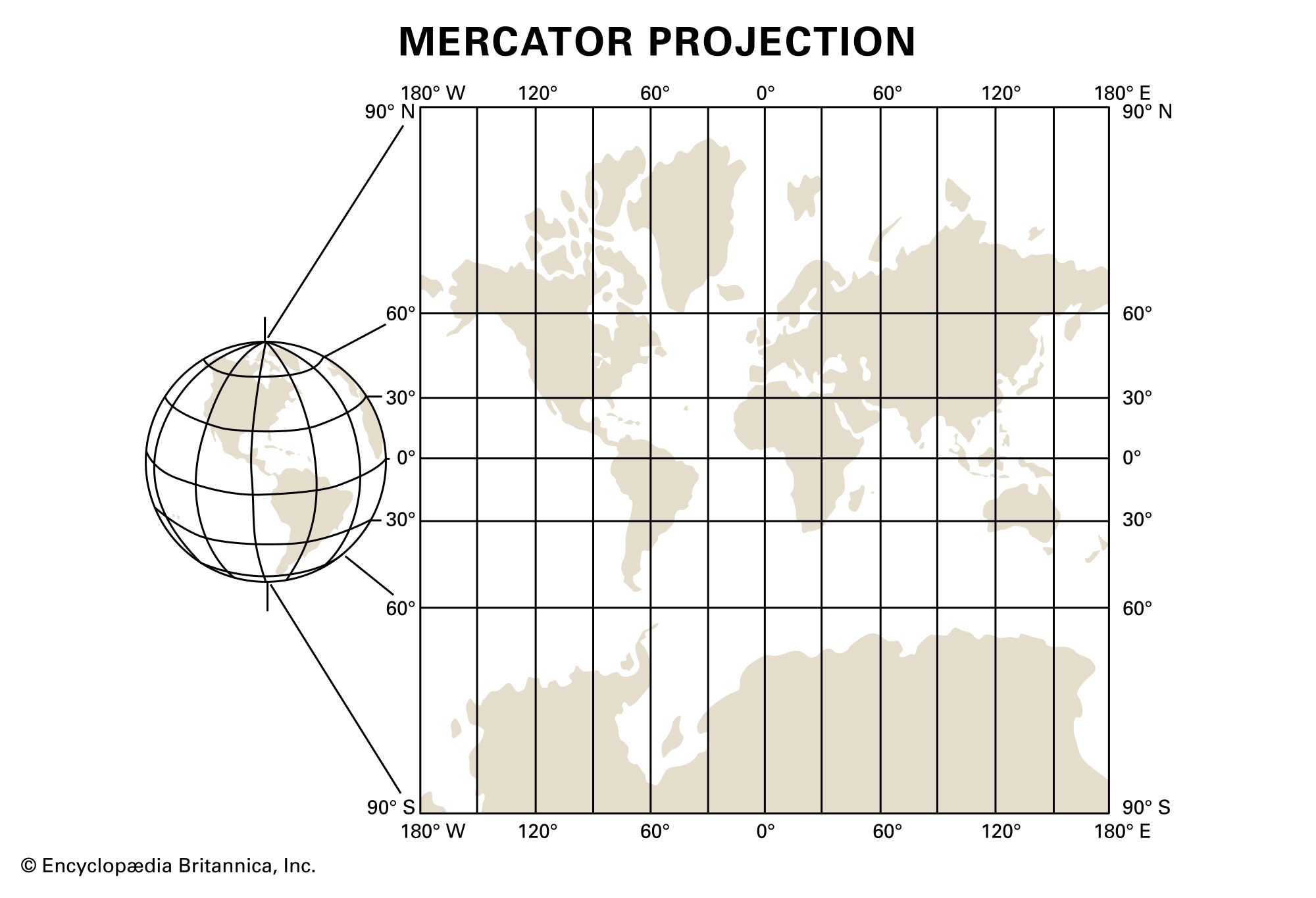
  • We live on a globe.
  • We like to create maps on flat pages.
  • We have to decide how to map things on a globe to a flat page.
  • Enter, projections.

Simple Features Maps

  • We’d often like to take spatial data that comes in the lat-long format given in the forested package and convert it to a format that accounts for the projection.

  • Often use the “simple features” standard produced by the Open Geospatial Consortium

    • R package: sf handles this type of data
    • Within ggplot2, geom_sf() and coord_sf() work with sf
  • In reality, this is the lat-long data, but encoded in a way that preserves projection information.

Making forested spatial

sf R package: simple features.

sf objects contain projection information and allow us to plot spatial data more accurately.

class(forested)
[1] "tbl_df"     "tbl"        "data.frame"
library(sf)
forested_sf <- forested %>%
  st_as_sf(coords = c("lon", "lat"), # columns in df that correspond to x and y coordinates
           crs = "EPSG:4269") # the projection the coordinates are in
class(forested_sf)
[1] "sf"         "tbl_df"     "tbl"        "data.frame"

Making forested spatial

glimpse(forested_sf)
Rows: 7,107
Columns: 19
$ forested         <fct> Yes, Yes, No, Yes, Yes, Yes, Yes, Yes, Yes, Yes, Yes,…
$ year             <dbl> 2005, 2005, 2005, 2005, 2005, 2005, 2005, 2005, 2005,…
$ elevation        <dbl> 881, 113, 164, 299, 806, 736, 636, 224, 52, 2240, 104…
$ eastness         <dbl> 90, -25, -84, 93, 47, -27, -48, -65, -62, -67, 96, -4…
$ northness        <dbl> 43, 96, 53, 34, -88, -96, 87, -75, 78, -74, -26, 86, …
$ roughness        <dbl> 63, 30, 13, 6, 35, 53, 3, 9, 42, 99, 51, 190, 95, 212…
$ tree_no_tree     <fct> Tree, Tree, Tree, No tree, Tree, Tree, No tree, Tree,…
$ dew_temp         <dbl> 0.04, 6.40, 6.06, 4.43, 1.06, 1.35, 1.42, 6.39, 6.50,…
$ precip_annual    <dbl> 466, 1710, 1297, 2545, 609, 539, 702, 1195, 1312, 103…
$ temp_annual_mean <dbl> 6.42, 10.64, 10.07, 9.86, 7.72, 7.89, 7.61, 10.45, 10…
$ temp_annual_min  <dbl> -8.32, 1.40, 0.19, -1.20, -5.98, -6.00, -5.76, 1.11, …
$ temp_annual_max  <dbl> 12.91, 15.84, 14.42, 15.78, 13.84, 14.66, 14.23, 15.3…
$ temp_january_min <dbl> -0.08, 5.44, 5.72, 3.95, 1.60, 1.12, 0.99, 5.54, 6.20…
$ vapor_min        <dbl> 78, 34, 49, 67, 114, 67, 67, 31, 60, 79, 172, 162, 70…
$ vapor_max        <dbl> 1194, 938, 754, 1164, 1254, 1331, 1275, 944, 892, 549…
$ canopy_cover     <dbl> 50, 79, 47, 42, 59, 36, 14, 27, 82, 12, 74, 66, 83, 6…
$ land_type        <fct> Tree, Tree, Tree, Tree, Tree, Tree, Non-tree vegetati…
$ county           <fct> Ferry, Thurston, Whatcom, Skamania, Stevens, Stevens,…
$ geometry         <POINT [°]> POINT (-118.6865 48.69537), POINT (-123.0825 47…
  • No longer has lon or lat columns.
  • Has a geometry column
    • This is a special type of column. Contains location and projection information.

Plotting forested_sf

ggplot(forested_sf, aes(color = forested)) +
  geom_sf(size = 0.5) + 
  scale_color_manual(values = c("forestgreen", "goldenrod3"))

ggplot(forested, aes(x = lon, y = lat, color = forested)) + 
  geom_point(size = 0.5) + 
  scale_color_manual(values = c("forestgreen", "goldenrod3"))

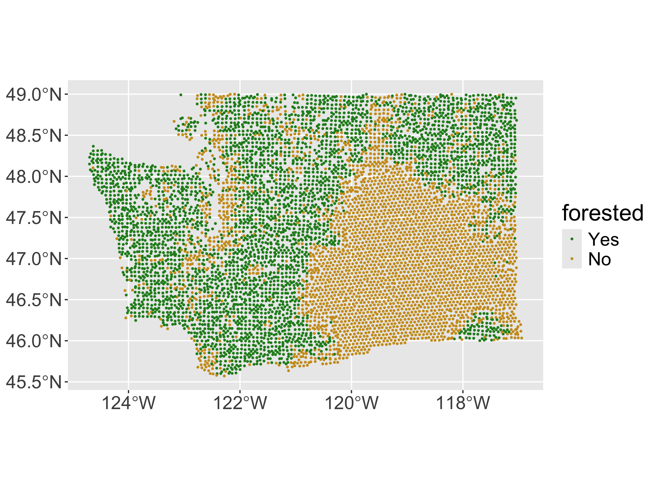
  • Preserves relative distances, rather than just plotting on the x/y plane.

Plotting forested_sf
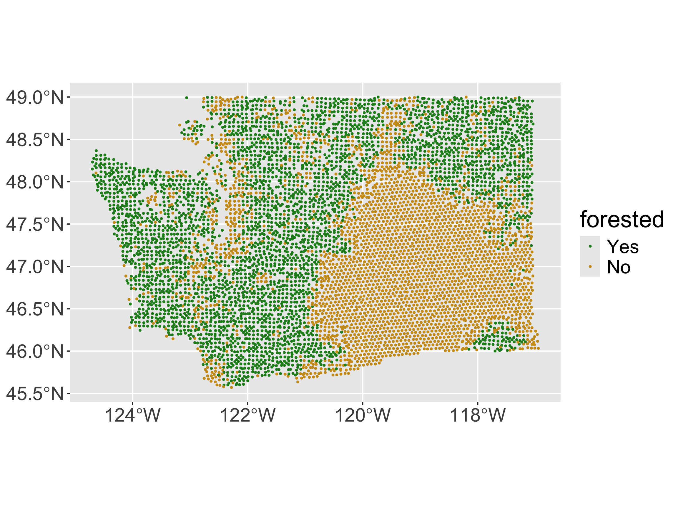
ggplot(forested_sf, aes(color = forested)) +
  geom_sf(size = 0.5) + 
  scale_color_manual(values = c("forestgreen", "goldenrod3"))

  • Implicitly, geom_sf() looks for a geometry column to set its “geometry” aesthetic to.

  • How can we add a base layer?

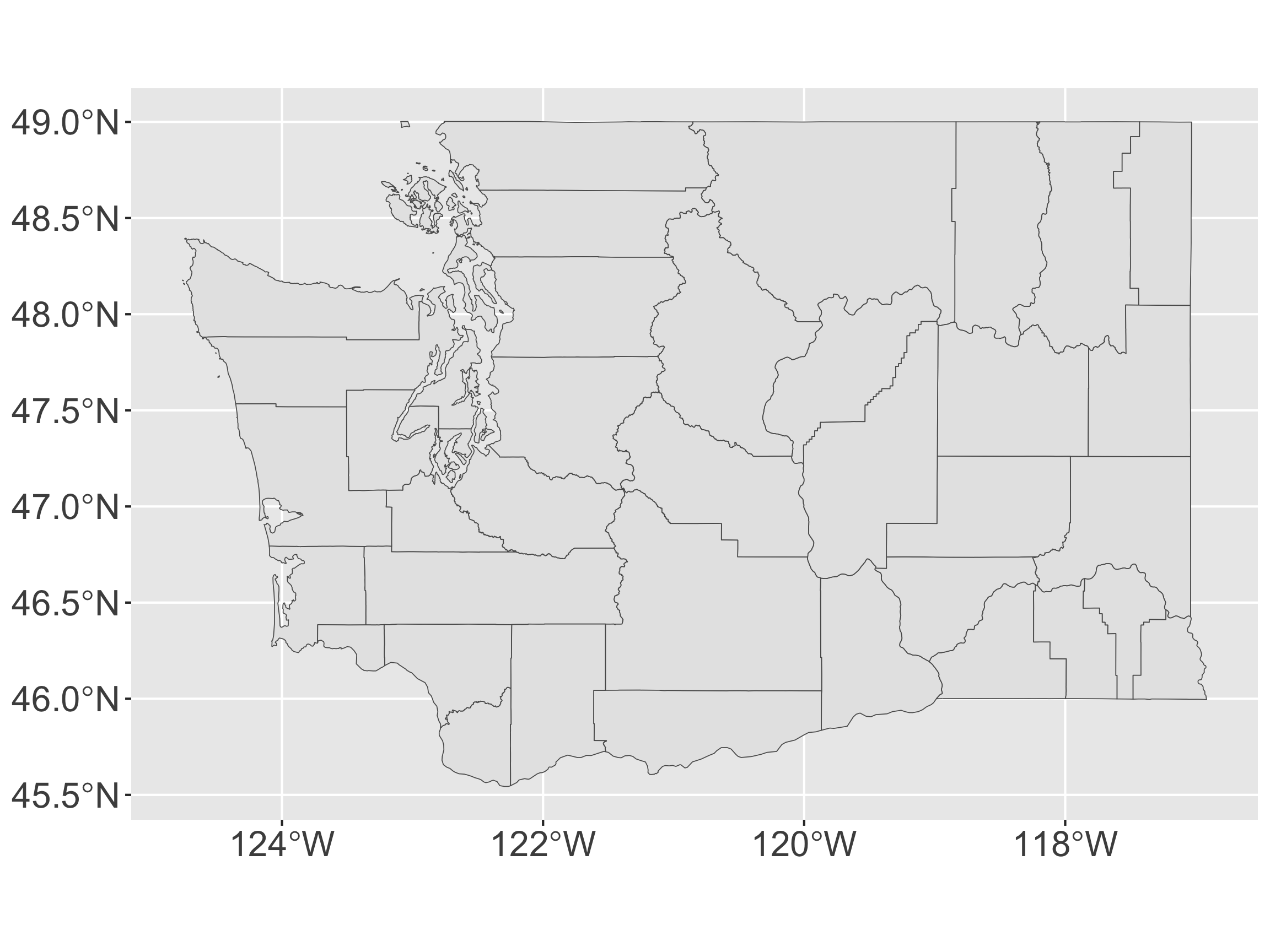
Polygon Maps

  • Want to draw various boundaries
    • EXs: Countries, states, counties, etc
  • polygon = closed area including the boundaries making up the area
tidycensus

  • Data from the US Census or American Community Survey
    • Comes in simple features format (using tigris)
    • Need to obtain an API key
api_key <- "insert key"
library(tidycensus)
options(tigris_use_cache = TRUE)
wa <- get_acs(state = "WA",  geography = "county",
              variables = "B19013_001",
              geometry = TRUE, key = api_key) 

What is the structure of wa?

class(wa)
[1] "sf"         "data.frame"
head(wa$geometry)
Geometry set for 6 features 
Geometry type: MULTIPOLYGON
Dimension:     XY
Bounding box:  xmin: -123.3727 ymin: 46.38346 xmax: -117.43 ymax: 49.00084
Geodetic CRS:  NAD83
First 5 geometries:
  • Row for each polygon
  • geometry contains the polygon object (borders of the county)

Compared to forested_sf

head(forested_sf$geometry)
Geometry set for 6 features 
Geometry type: POINT
Dimension:     XY
Bounding box:  xmin: -123.0825 ymin: 45.80776 xmax: -117.7224 ymax: 48.77132
Geodetic CRS:  NAD83
First 5 geometries:
  • Row for each point, geometry contains the point object (center of the plot)

Adding a base layer to our original map
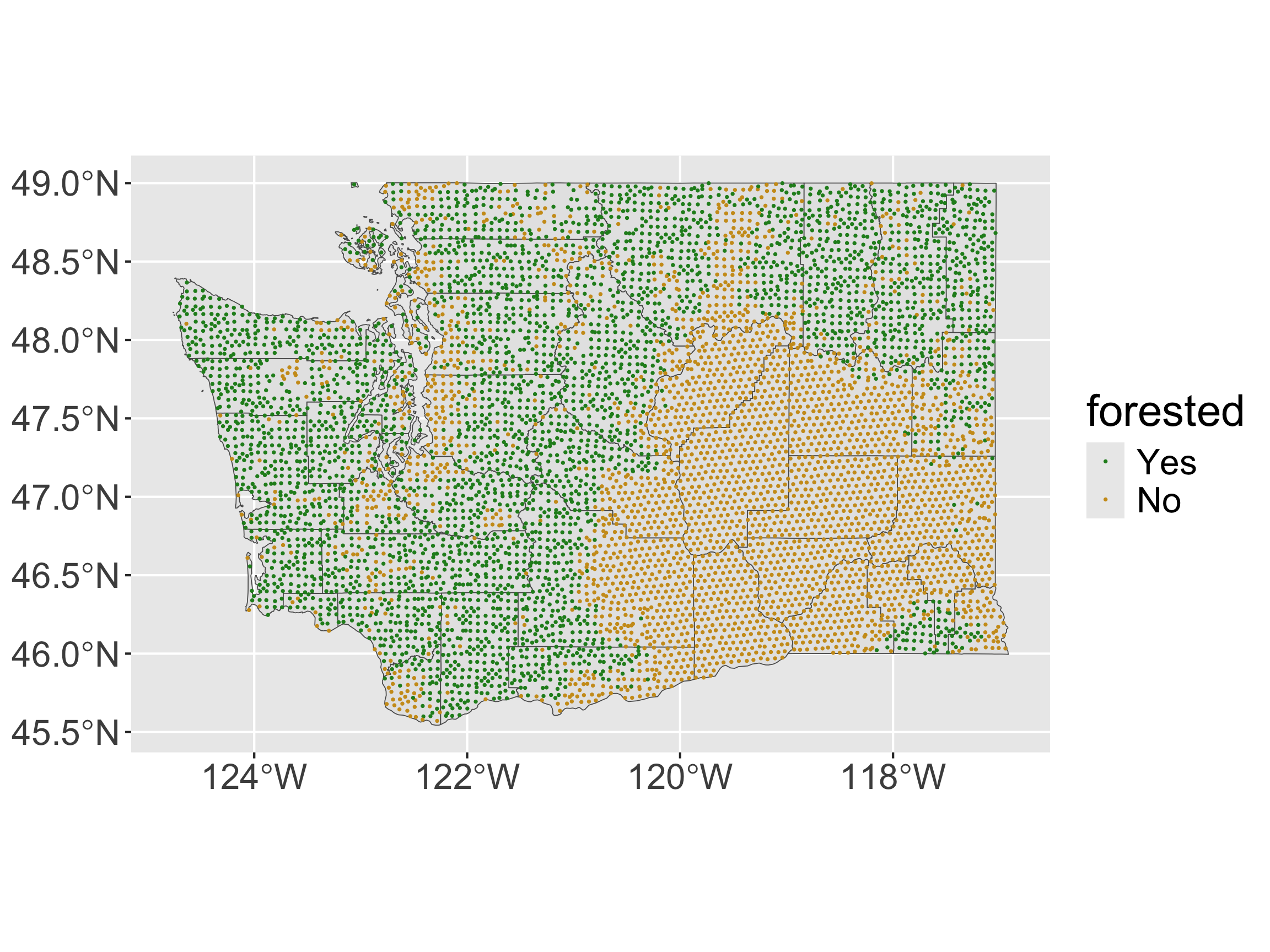
ggplot() +
  geom_sf(data = wa) + 
  geom_sf(data = forested_sf, aes(color = forested), size = 0.2) + 
  scale_color_manual(values = c("forestgreen", "goldenrod3"))

What if we’d like to map the proportion of forested plots in each county in WA?

forested_props <- forested %>%
  group_by(county) %>%
  summarize(prop_forested = mean(forested == "Yes"))

forested_props
# A tibble: 39 × 2
   county   prop_forested
   <fct>            <dbl>
 1 Adams           0     
 2 Asotin          0.239 
 3 Benton          0     
 4 Chelan          0.741 
 5 Clallam         0.928 
 6 Clark           0.535 
 7 Columbia        0.347 
 8 Cowlitz         0.887 
 9 Douglas         0.0109
10 Ferry           0.908 
# ℹ 29 more rows
  • Want to make a chloropleth map.

Need to join with wa… 🤔

head(forested_props)
# A tibble: 6 × 2
  county  prop_forested
  <fct>           <dbl>
1 Adams           0    
2 Asotin          0.239
3 Benton          0    
4 Chelan          0.741
5 Clallam         0.928
6 Clark           0.535
head(wa)
Simple feature collection with 6 features and 5 fields
Geometry type: MULTIPOLYGON
Dimension:     XY
Bounding box:  xmin: -123.3727 ymin: 46.38346 xmax: -117.43 ymax: 49.00084
Geodetic CRS:  NAD83
  GEOID                        NAME   variable estimate  moe
1 53067 Thurston County, Washington B19013_001    93985 1815
2 53029   Island County, Washington B19013_001    88358 2918
3 53041    Lewis County, Washington B19013_001    69690 3237
4 53065  Stevens County, Washington B19013_001    67405 3514
5 53017  Douglas County, Washington B19013_001    80374 4122
6 53055 San Juan County, Washington B19013_001    83682 4942
                        geometry
1 MULTIPOLYGON (((-123.2009 4...
2 MULTIPOLYGON (((-122.5389 4...
3 MULTIPOLYGON (((-123.371 46...
4 MULTIPOLYGON (((-118.4024 4...
5 MULTIPOLYGON (((-120.3178 4...
6 MULTIPOLYGON (((-122.7666 4...
  • Want by = c("county" = "NAME"). Why won’t this work??

Solution: our trick from last time!

wa <- wa %>%
  separate_wider_delim(cols = "NAME", 
                       delim = " County",
                       names = c("short_name", NA)) 
head(wa$short_name)
[1] "Thurston" "Island"   "Lewis"    "Stevens"  "Douglas"  "San Juan"
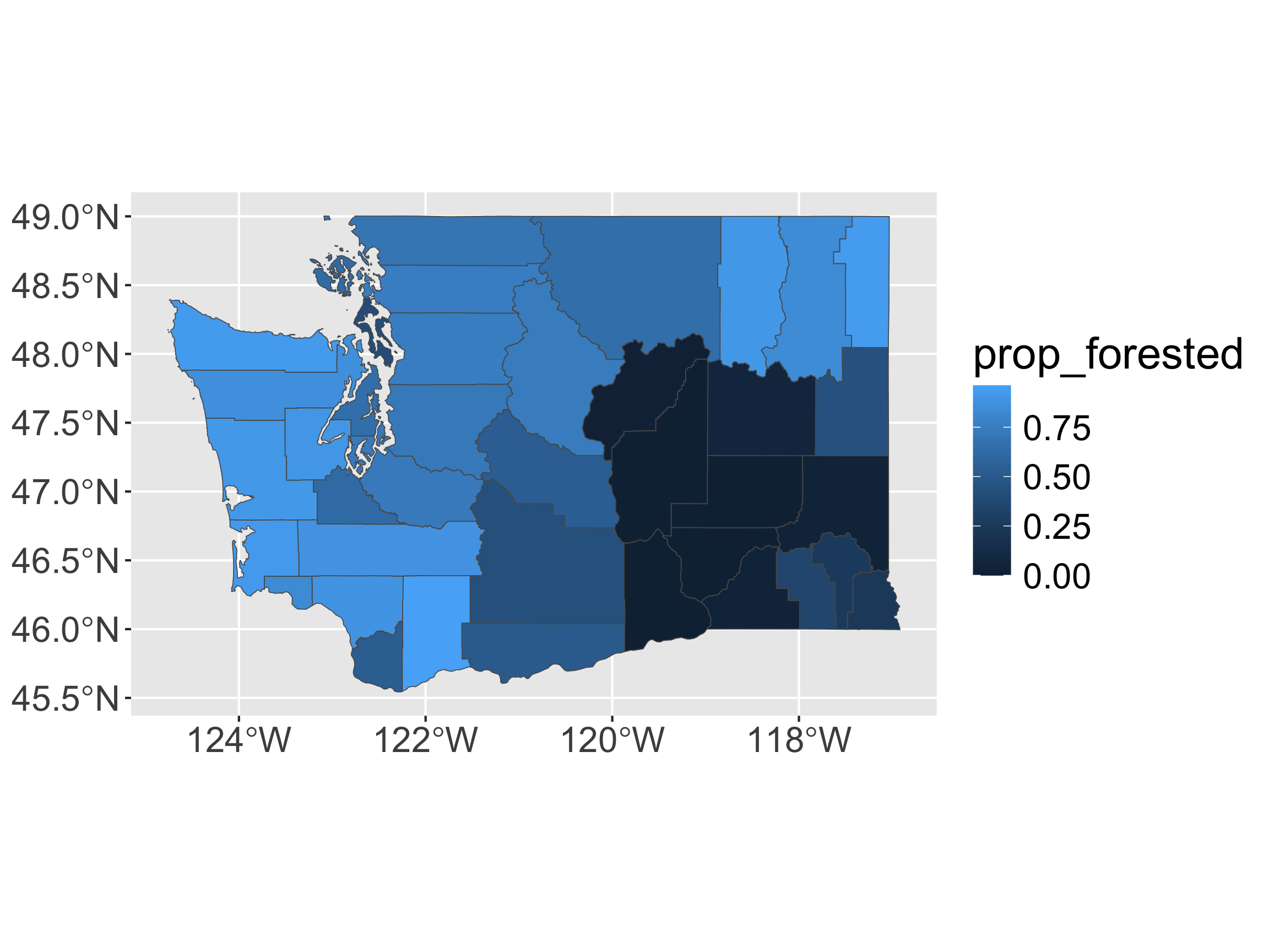

# join
left_join(forested_props,
          wa,
          by = c("county" = "short_name")) %>% 
  # make R remember this is an sf object 
  # (R keeps the class of the primary dataset)
  st_as_sf() %>% 
  ggplot(aes(fill = prop_forested)) + 
  geom_sf() 

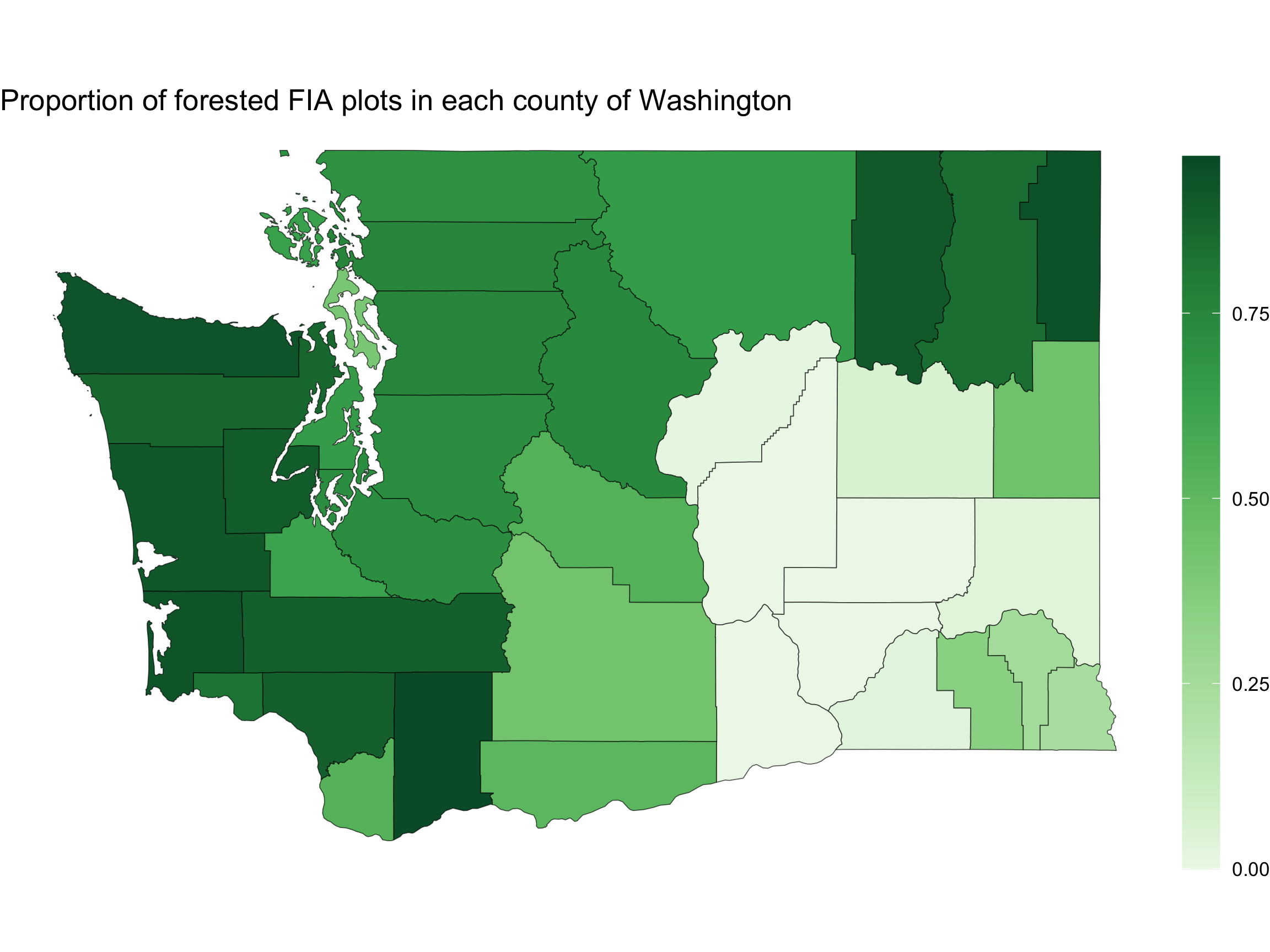
Some mapping suggestions

# join
left_join(forested_props,
          wa,
          by = c("county" = "short_name")) %>% 
  # make R remember this is an sf object 
  # (R keeps the class of the primary dataset)
  st_as_sf() %>% 
  ggplot(aes(fill = prop_forested)) + 
  geom_sf() + 
  scale_fill_distiller(type = "seq", 
                       palette = "Greens", 
                       direction = 1) +
  labs(title = "Proportion of forested FIA plots in each county of Washington",
       fill = "") +
  theme_void() +
  theme(legend.position = "right",
        legend.key.height = unit(0.9, "in"))
Back to tidycensus

Recall our call to get county polygons:

api_key <- "insert key"
library(tidycensus)
options(tigris_use_cache = TRUE)
wa <- get_acs(state = "WA",  geography = "county",
              variables = "B19013_001",
              geometry = TRUE, key = api_key) 
  • What is going on with variables = "B19013_001"?

Back to tidycensus

B19013_001 = Median Household Income

vars <- load_variables(2021, "acs5", cache = FALSE)
vars
# A tibble: 27,886 × 4
   name        label                                    concept        geography
   <chr>       <chr>                                    <chr>          <chr>    
 1 B01001A_001 Estimate!!Total:                         SEX BY AGE (W… tract    
 2 B01001A_002 Estimate!!Total:!!Male:                  SEX BY AGE (W… tract    
 3 B01001A_003 Estimate!!Total:!!Male:!!Under 5 years   SEX BY AGE (W… tract    
 4 B01001A_004 Estimate!!Total:!!Male:!!5 to 9 years    SEX BY AGE (W… tract    
 5 B01001A_005 Estimate!!Total:!!Male:!!10 to 14 years  SEX BY AGE (W… tract    
 6 B01001A_006 Estimate!!Total:!!Male:!!15 to 17 years  SEX BY AGE (W… tract    
 7 B01001A_007 Estimate!!Total:!!Male:!!18 and 19 years SEX BY AGE (W… tract    
 8 B01001A_008 Estimate!!Total:!!Male:!!20 to 24 years  SEX BY AGE (W… tract    
 9 B01001A_009 Estimate!!Total:!!Male:!!25 to 29 years  SEX BY AGE (W… tract    
10 B01001A_010 Estimate!!Total:!!Male:!!30 to 34 years  SEX BY AGE (W… tract    
# ℹ 27,876 more rows

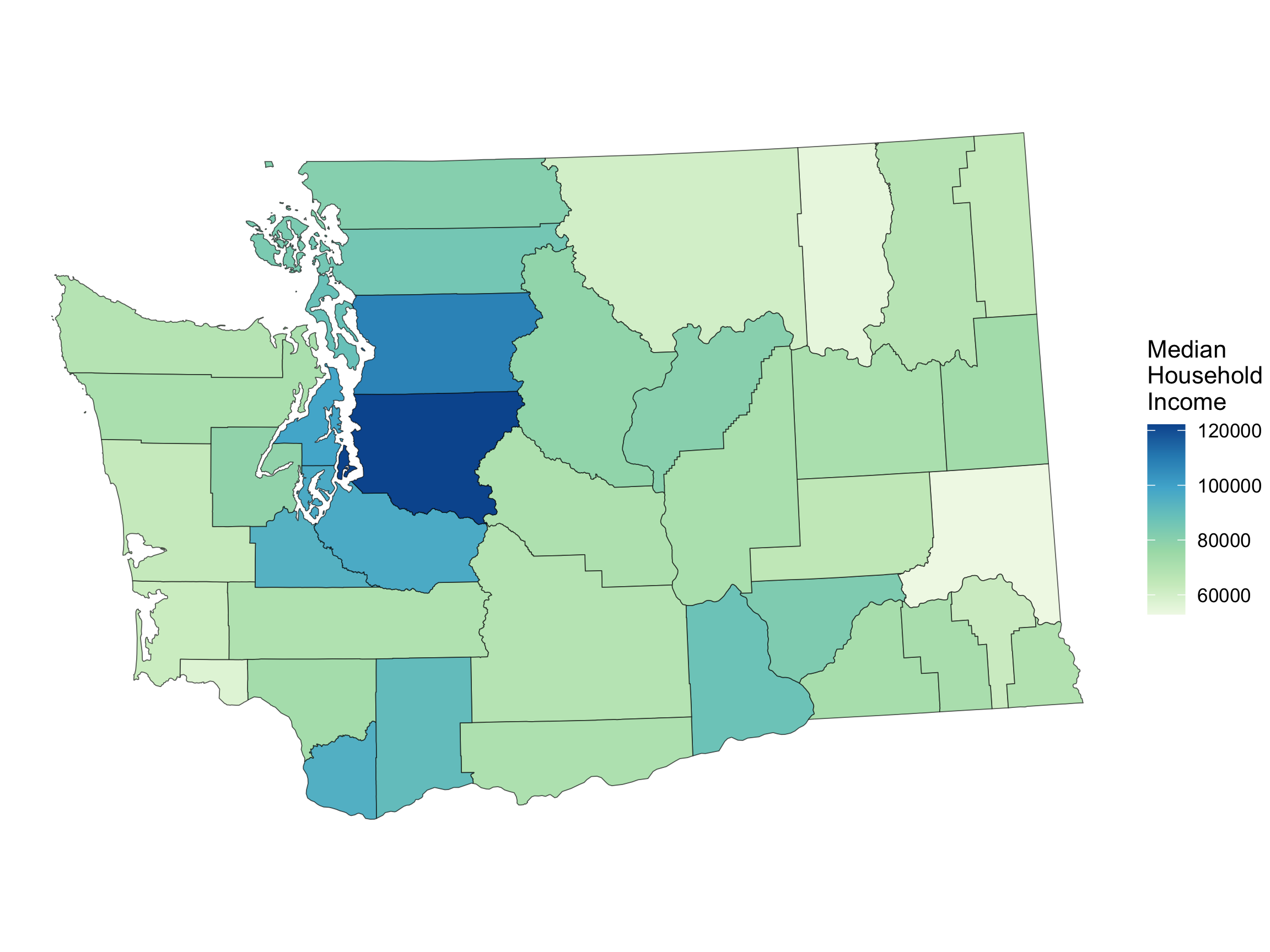
Choropleth Map Showing Median Household Income
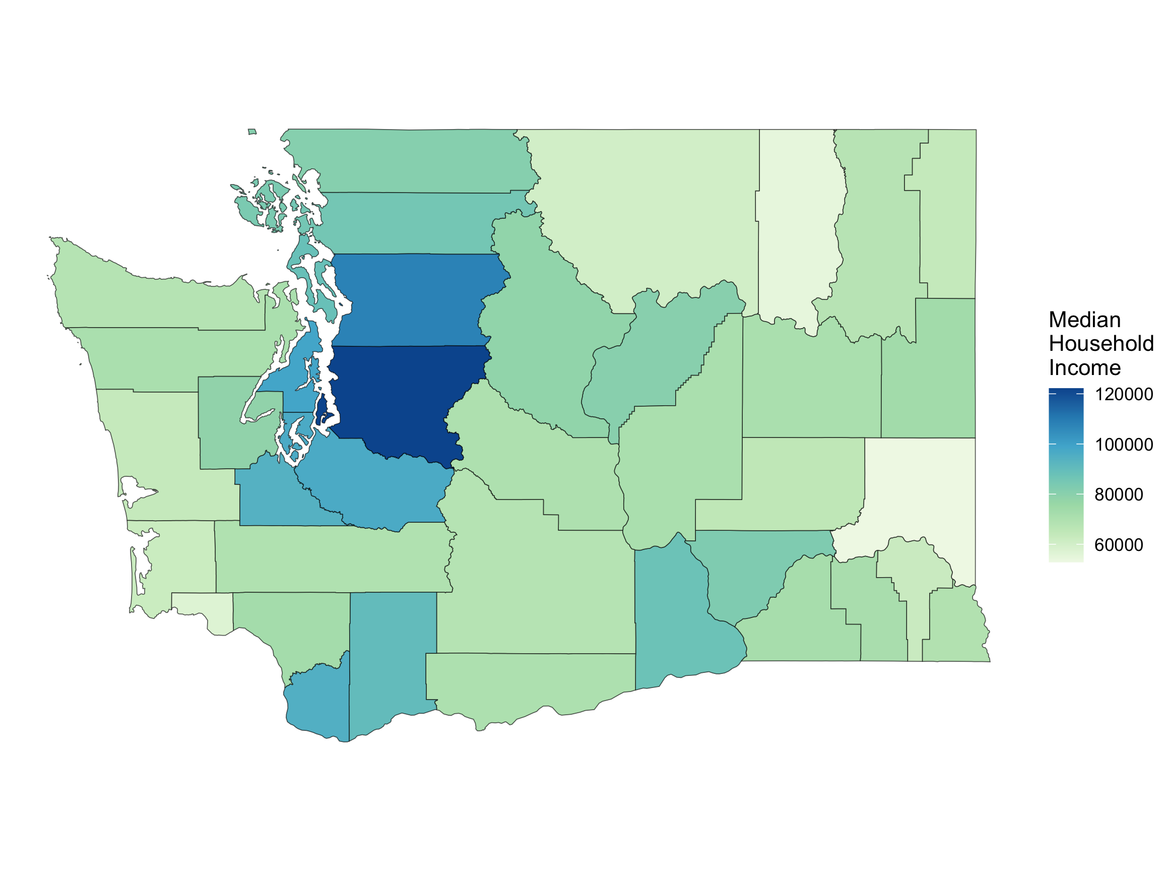
ggplot(data = wa, 
       mapping = 
         aes(geometry = geometry,
             fill = estimate)) + 
  geom_sf() +
  scale_fill_distiller(
   name = "Median \nHousehold \nIncome",
   direction = 1, type = "seq", palette = 4) +
  theme_void()

Choropleth Map

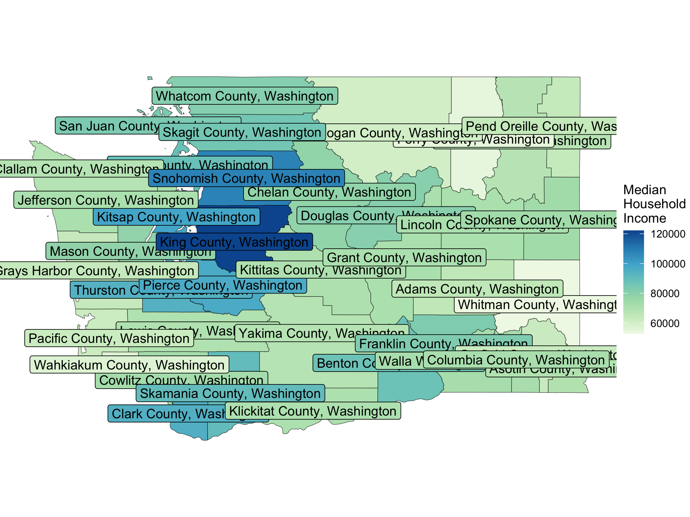
ggplot(data = wa, 
       mapping = 
         aes(geometry = geometry,
             fill = estimate)) + 
  geom_sf() +
  geom_sf_label(aes(label = NAME)) +
  scale_fill_distiller(
   name = "Median \nHousehold \nIncome",
   direction = 1, type = "seq", palette = 4) +
  theme_void()

  • How should we modify the code if we don’t want the labels to be colored differently?

Choropleth Map
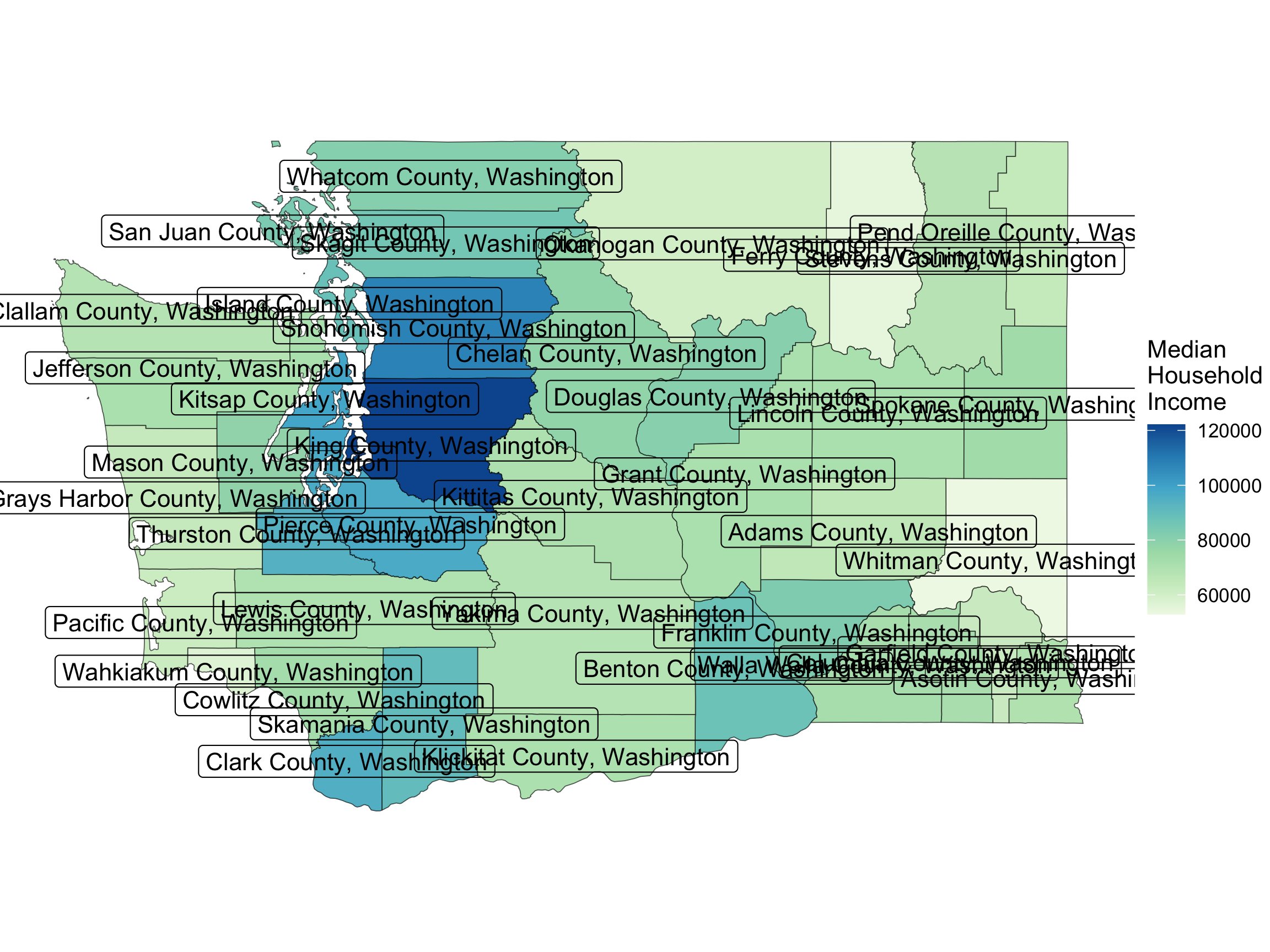
ggplot(data = wa, 
       mapping = 
         aes(geometry = geometry)) + 
  geom_sf(mapping = 
            aes(fill = estimate)) +
  geom_sf_label(aes(label = NAME)) +
  scale_fill_distiller(
   name = "Median \nHousehold \nIncome",
   direction = 1, type = "seq", palette = 4) +
  theme_void()
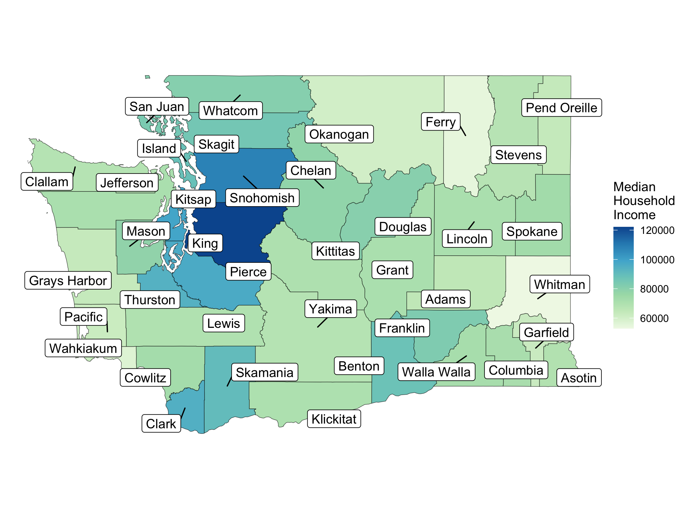
  • Fixes for crowding?

This time, use the stringr Package

This time, for fun, we will use the stringr package to get the same result as we did with the tidyr package:

One way:

wa <- wa %>%
  mutate(short_name = 
           str_replace_all(
             NAME, 
             pattern = " County, Washington", 
             replacement = ""
            )
         )
head(wa$short_name)
[1] "Thurston" "Island"   "Lewis"    "Stevens"  "Douglas"  "San Juan"

Another way:

wa <- wa %>%
  mutate(short_name = 
           str_sub(NAME,
                   start = 1, 
                   end = -20))
head(wa$short_name)
[1] "Thurston" "Island"   "Lewis"    "Stevens"  "Douglas"  "San Juan"

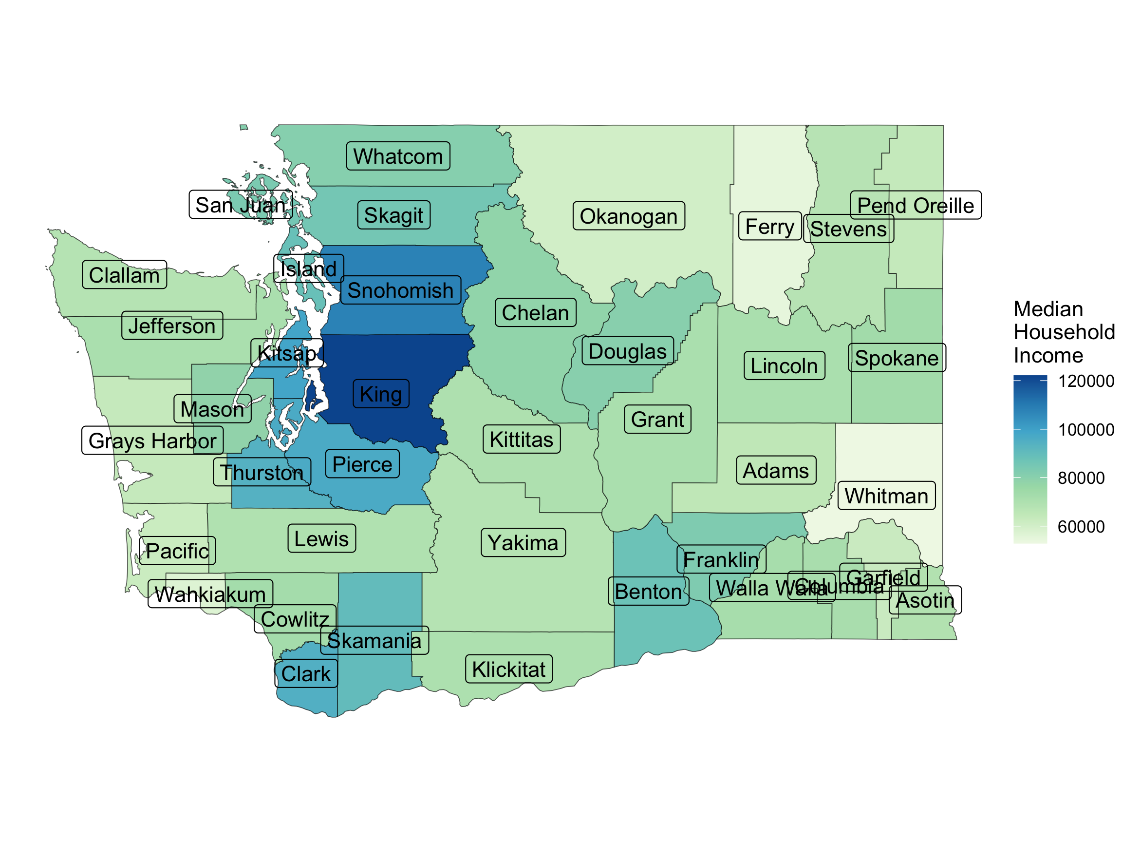
Choropleth Map

ggplot(data = wa, 
       mapping = 
         aes(geometry = geometry)) + 
  geom_sf(mapping = 
            aes(fill = estimate)) +
  geom_sf_label(aes(label = short_name)) +
  scale_fill_distiller(
   name = "Median \nHousehold \nIncome",
   direction = 1, type = "seq", palette = 4) +
  theme_void()
  • Fixes for crowding?

Choropleth Map

#devtools::install_github("yutannihilation/ggsflabel")
library(ggsflabel)
ggplot(data = wa, 
       mapping = 
         aes(geometry = geometry)) + 
  geom_sf(mapping = 
            aes(fill = estimate)) +
  geom_sf_label_repel(aes(label = short_name),
                      force = 40) +
  scale_fill_distiller(
   name = "Median \nHousehold \nIncome",
   direction = 1, type = "seq", palette = 4) +
  theme_void()

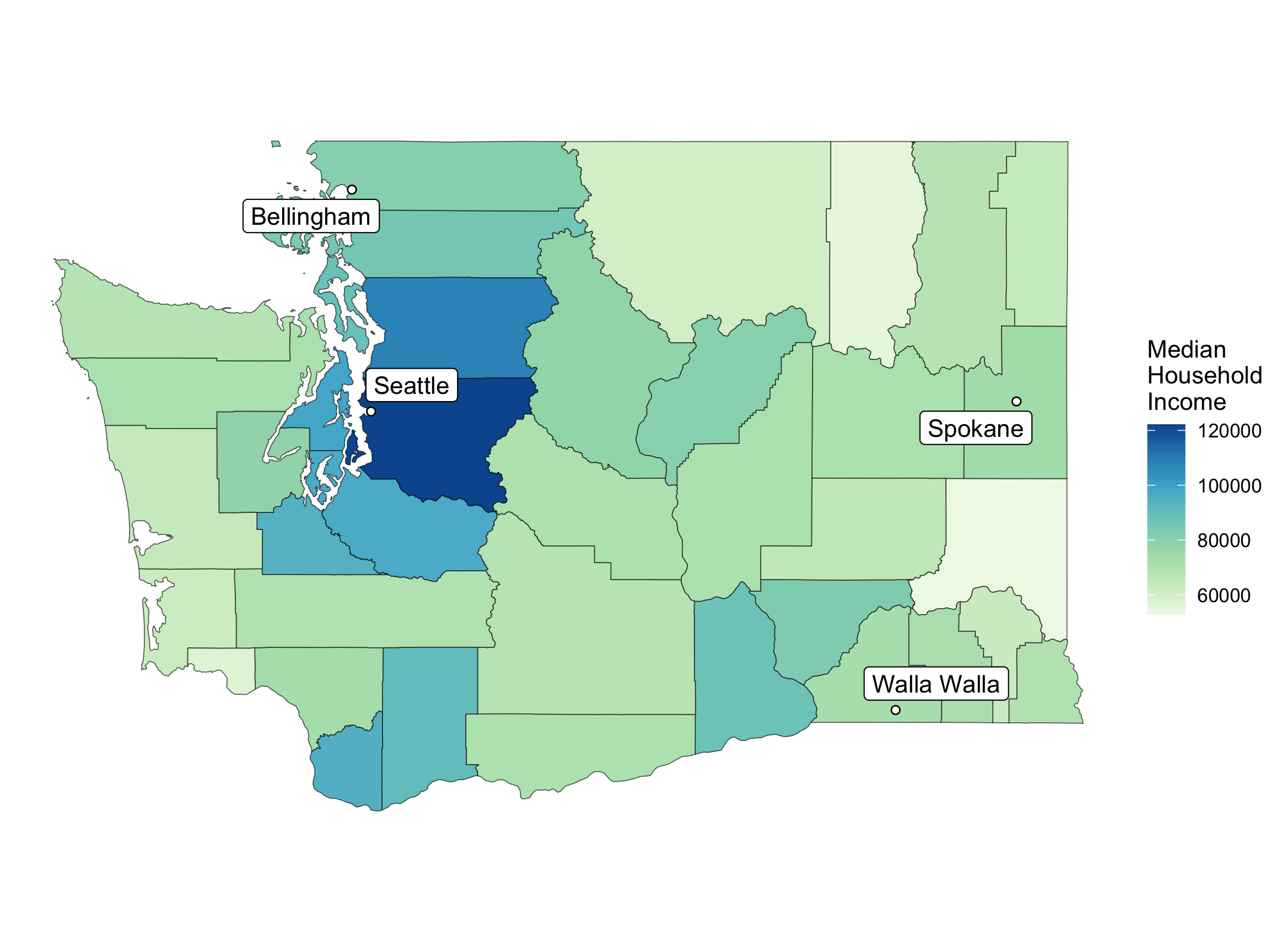
Can Add Information from Another Dataset

wa_cities <- data_frame(city = c("Seattle", "Bellingham", 
                                 "Walla Walla", "Spokane"),
                        lat = c(47.6061, 48.7519, 46.0646, 47.6580),
                        long = c(-122.3328, -122.4787,
                                 -118.3430, -117.4235))
wa_cities
# A tibble: 4 × 3
  city          lat  long
  <chr>       <dbl> <dbl>
1 Seattle      47.6 -122.
2 Bellingham   48.8 -122.
3 Walla Walla  46.1 -118.
4 Spokane      47.7 -117.

Can Add Information from Another Dataset

library(ggrepel)
ggplot() + 
  geom_sf(data = wa,
          mapping = 
            aes(geometry = geometry, 
                fill = estimate)) +
  geom_point(data = wa_cities,
             mapping = aes(x = long,
                           y = lat),
             shape = 21,
             fill = "white",
             color = "black") +
  geom_label_repel(data = wa_cities,
                   mapping = 
                     aes(x = long,
                         y = lat,
                         label = city)) +
  scale_fill_distiller(
   name = "Median \nHousehold \nIncome",
   direction = 1, type = "seq", palette = 4) +
  theme_void()

Coordinate Reference System

Census defaults to NAD 1983 (EPSG: 4269) for its coordinate reference system

wa
Simple feature collection with 39 features and 6 fields
Geometry type: MULTIPOLYGON
Dimension:     XY
Bounding box:  xmin: -124.7631 ymin: 45.54354 xmax: -116.916 ymax: 49.00249
Geodetic CRS:  NAD83
First 10 features:
   GEOID                        NAME   variable estimate  moe
1  53067 Thurston County, Washington B19013_001    93985 1815
2  53029   Island County, Washington B19013_001    88358 2918
3  53041    Lewis County, Washington B19013_001    69690 3237
4  53065  Stevens County, Washington B19013_001    67405 3514
5  53017  Douglas County, Washington B19013_001    80374 4122
6  53055 San Juan County, Washington B19013_001    83682 4942
7  53035   Kitsap County, Washington B19013_001    98546 2118
8  53011    Clark County, Washington B19013_001    94948 1484
9  53045    Mason County, Washington B19013_001    78359 4033
10 53053   Pierce County, Washington B19013_001    96632 1316
                         geometry short_name
1  MULTIPOLYGON (((-123.2009 4...   Thurston
2  MULTIPOLYGON (((-122.5389 4...     Island
3  MULTIPOLYGON (((-123.371 46...      Lewis
4  MULTIPOLYGON (((-118.4024 4...    Stevens
5  MULTIPOLYGON (((-120.3178 4...    Douglas
6  MULTIPOLYGON (((-122.7666 4...   San Juan
7  MULTIPOLYGON (((-122.5049 4...     Kitsap
8  MULTIPOLYGON (((-122.796 45...      Clark
9  MULTIPOLYGON (((-123.5059 4...      Mason
10 MULTIPOLYGON (((-122.6406 4...     Pierce

Coordinate Reference System

Census defaults to NAD 1983 (EPSG: 4269) for its coordinate reference system

library(sf)
st_crs(wa)
Coordinate Reference System:
  User input: NAD83 
  wkt:
GEOGCRS["NAD83",
    DATUM["North American Datum 1983",
        ELLIPSOID["GRS 1980",6378137,298.257222101,
            LENGTHUNIT["metre",1]]],
    PRIMEM["Greenwich",0,
        ANGLEUNIT["degree",0.0174532925199433]],
    CS[ellipsoidal,2],
        AXIS["latitude",north,
            ORDER[1],
            ANGLEUNIT["degree",0.0174532925199433]],
        AXIS["longitude",east,
            ORDER[2],
            ANGLEUNIT["degree",0.0174532925199433]],
    ID["EPSG",4269]]

Coordinate Reference System

  • You can choose a more local coordinate reference system depending on your map extent.

  • Projection EPSG:32610 = UTM zone 10N, good for the PNW.

wa_transf <- sf::st_transform(wa, "EPSG:32610")
wa_transf
Simple feature collection with 39 features and 6 fields
Geometry type: MULTIPOLYGON
Dimension:     XY
Bounding box:  xmin: 368934 ymin: 5043576 xmax: 971107.1 ymax: 5444546
Projected CRS: WGS 84 / UTM zone 10N
First 10 features:
   GEOID                        NAME   variable estimate  moe
1  53067 Thurston County, Washington B19013_001    93985 1815
2  53029   Island County, Washington B19013_001    88358 2918
3  53041    Lewis County, Washington B19013_001    69690 3237
4  53065  Stevens County, Washington B19013_001    67405 3514
5  53017  Douglas County, Washington B19013_001    80374 4122
6  53055 San Juan County, Washington B19013_001    83682 4942
7  53035   Kitsap County, Washington B19013_001    98546 2118
8  53011    Clark County, Washington B19013_001    94948 1484
9  53045    Mason County, Washington B19013_001    78359 4033
10 53053   Pierce County, Washington B19013_001    96632 1316
                         geometry short_name
1  MULTIPOLYGON (((484730.4 52...   Thurston
2  MULTIPOLYGON (((534255.1 53...     Island
3  MULTIPOLYGON (((471689.1 51...      Lewis
4  MULTIPOLYGON (((842746.2 53...    Stevens
5  MULTIPOLYGON (((702143.6 52...    Douglas
6  MULTIPOLYGON (((517173.5 53...   San Juan
7  MULTIPOLYGON (((537252.9 52...     Kitsap
8  MULTIPOLYGON (((515848.8 50...      Clark
9  MULTIPOLYGON (((461911.4 52...      Mason
10 MULTIPOLYGON (((527244.4 52...     Pierce

Different CRS -> Different Looking Map
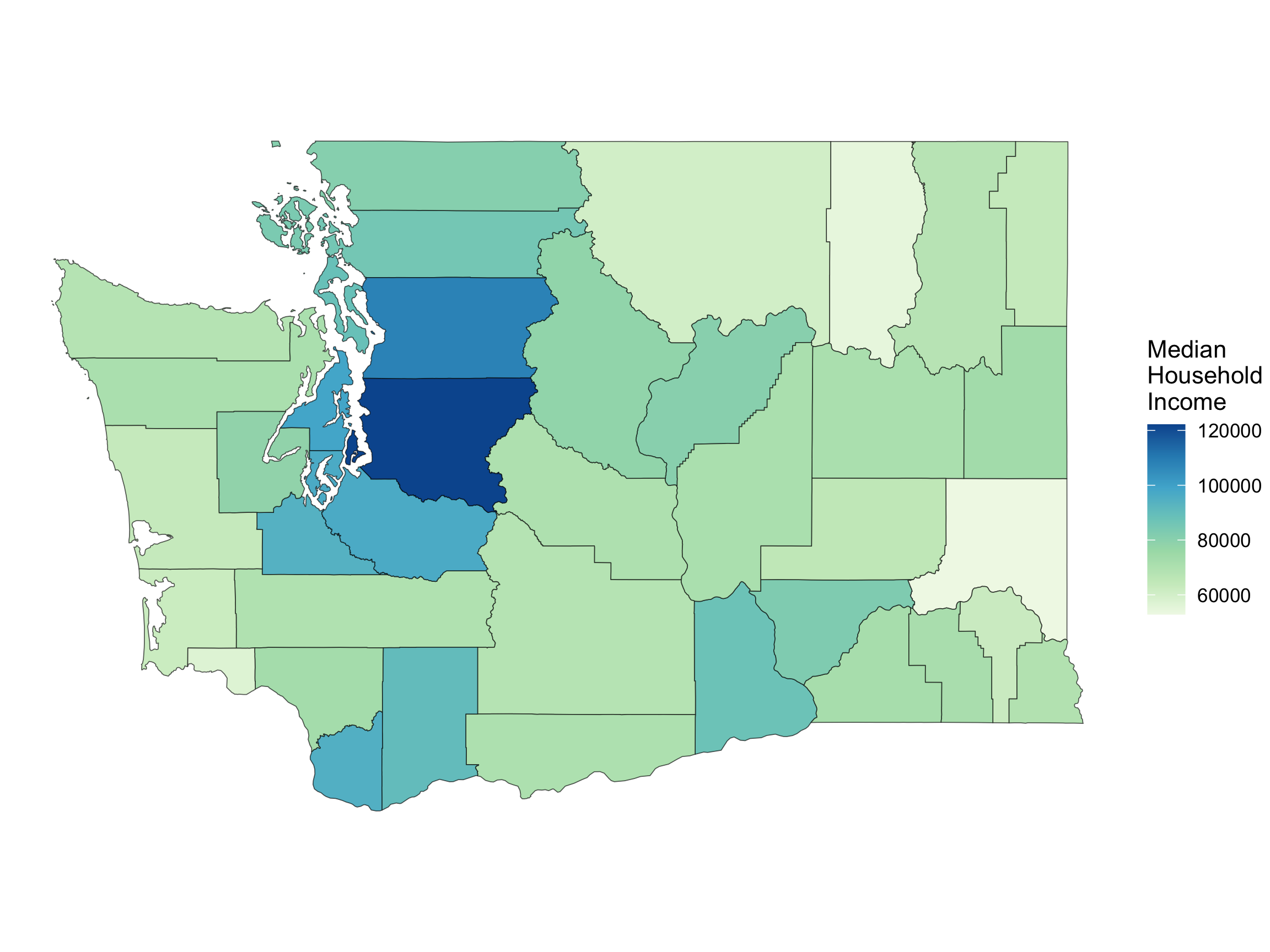
ggplot() + 
  geom_sf(data = wa,
          mapping = 
            aes(geometry = geometry, 
                fill = estimate)) +
  coord_sf() +
  scale_fill_distiller(
   name = "Median \nHousehold \nIncome",
   direction = 1, type = "seq", palette = 4) +
  theme_void()

ggplot() + 
  geom_sf(data = wa_transf,
          mapping = 
            aes(geometry = geometry, 
                fill = estimate)) +
  coord_sf() +
  scale_fill_distiller(
   name = "Median \nHousehold \nIncome",
   direction = 1, type = "seq", palette = 4) +
  theme_void()

Cartograms

Scale polygons by a variable.
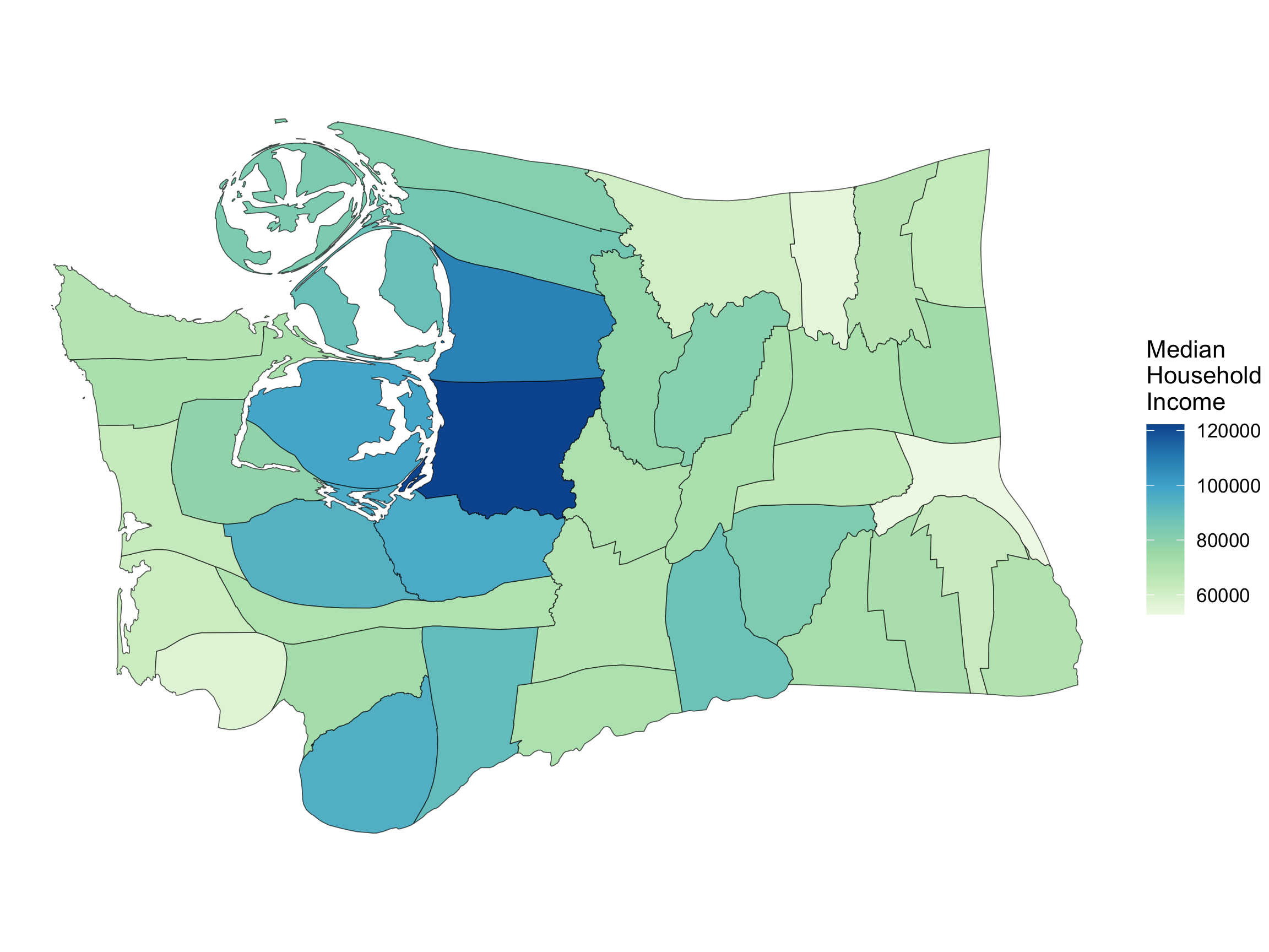
library(cartogram)
wa_carto <- cartogram_cont(wa_transf, 
                           weight = "estimate")

ggplot() + 
  geom_sf(data = wa_carto,
          mapping = 
            aes(geometry = geometry, 
                fill = estimate)) +
  coord_sf() +
  scale_fill_distiller(
   name = "Median \nHousehold \nIncome",
   direction = 1, type = "seq", palette = 4) +
  theme_void()
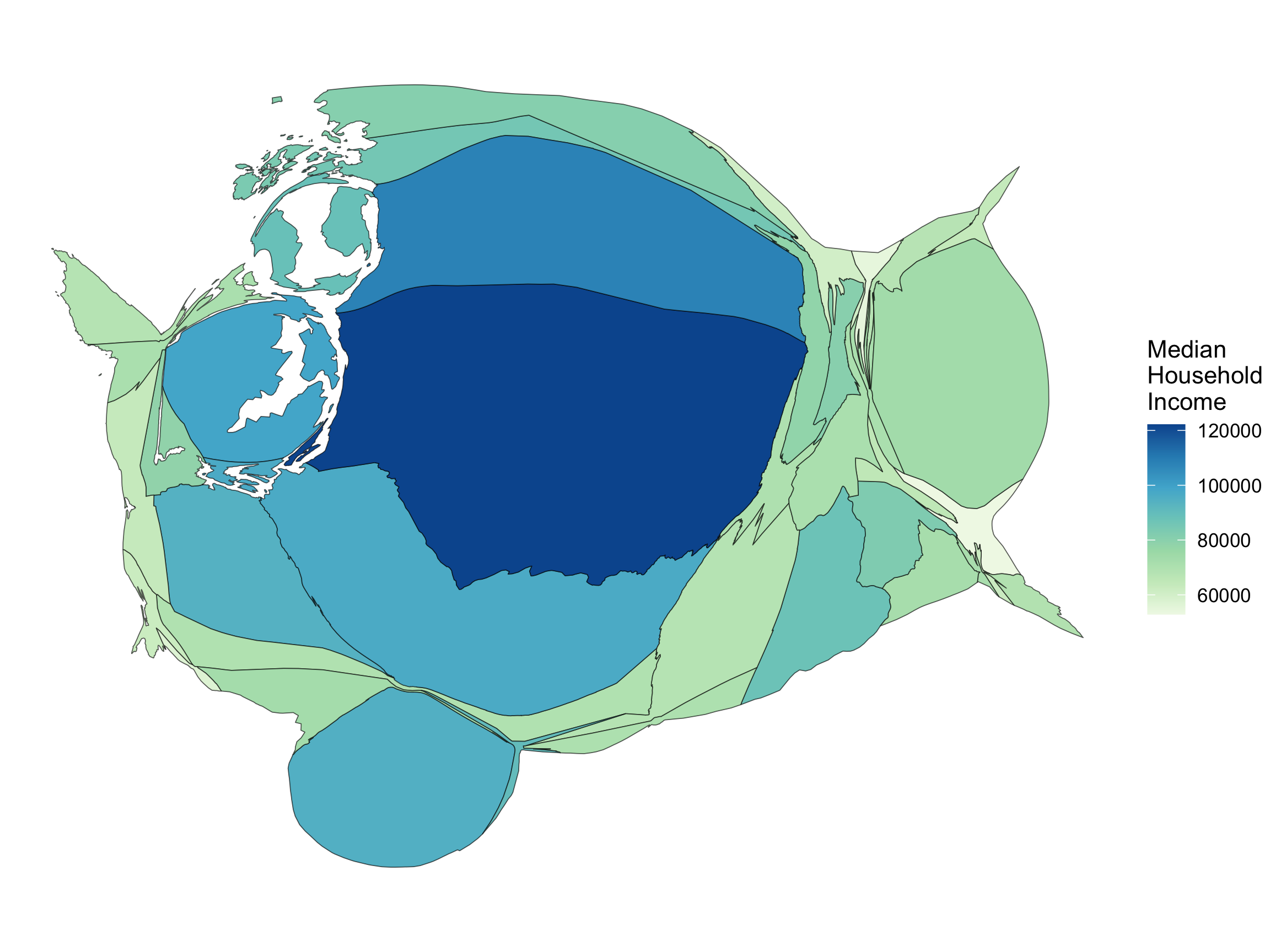
Cartograms

Often scaled by a population size type variable.

wa_pop <- get_decennial(state = "WA", geography = "county",
                        variables = "P001001", year = 2010, key = api_key)

wa_transf_pop <- inner_join(wa_transf, wa_pop, by = c("GEOID" = "GEOID"))
wa_transf_pop
Simple feature collection with 39 features and 9 fields
Geometry type: MULTIPOLYGON
Dimension:     XY
Bounding box:  xmin: 368934 ymin: 5043576 xmax: 971107.1 ymax: 5444546
Projected CRS: WGS 84 / UTM zone 10N
First 10 features:
   GEOID                      NAME.x variable.x estimate  moe short_name
1  53067 Thurston County, Washington B19013_001    93985 1815   Thurston
2  53029   Island County, Washington B19013_001    88358 2918     Island
3  53041    Lewis County, Washington B19013_001    69690 3237      Lewis
4  53065  Stevens County, Washington B19013_001    67405 3514    Stevens
5  53017  Douglas County, Washington B19013_001    80374 4122    Douglas
6  53055 San Juan County, Washington B19013_001    83682 4942   San Juan
7  53035   Kitsap County, Washington B19013_001    98546 2118     Kitsap
8  53011    Clark County, Washington B19013_001    94948 1484      Clark
9  53045    Mason County, Washington B19013_001    78359 4033      Mason
10 53053   Pierce County, Washington B19013_001    96632 1316     Pierce
                        NAME.y variable.y  value                       geometry
1  Thurston County, Washington    P001001 252264 MULTIPOLYGON (((484730.4 52...
2    Island County, Washington    P001001  78506 MULTIPOLYGON (((534255.1 53...
3     Lewis County, Washington    P001001  75455 MULTIPOLYGON (((471689.1 51...
4   Stevens County, Washington    P001001  43531 MULTIPOLYGON (((842746.2 53...
5   Douglas County, Washington    P001001  38431 MULTIPOLYGON (((702143.6 52...
6  San Juan County, Washington    P001001  15769 MULTIPOLYGON (((517173.5 53...
7    Kitsap County, Washington    P001001 251133 MULTIPOLYGON (((537252.9 52...
8     Clark County, Washington    P001001 425363 MULTIPOLYGON (((515848.8 50...
9     Mason County, Washington    P001001  60699 MULTIPOLYGON (((461911.4 52...
10   Pierce County, Washington    P001001 795225 MULTIPOLYGON (((527244.4 52...

Cartograms

Often scaled by a population size type variable.

wa_transf_pop <- wa_transf_pop %>%
  rename(population_size = value, 
         median_income = estimate)

wa_transf_pop <- cartogram_cont(
  wa_transf_pop,                                 
  weight = "population_size"
  )

ggplot() + 
  geom_sf(data = wa_transf_pop,
          mapping = 
            aes(geometry = geometry, 
                fill = median_income)) +
  coord_sf() +
  scale_fill_distiller(
   name = "Median \nHousehold \nIncome",
   direction = 1, type = "seq", palette = 4) +
  theme_void()

New Dataset

State Level Information

library(Lock5Data)
glimpse(USStates)
Rows: 50
Columns: 22
$ State            <fct> Alabama, Alaska, Arizona, Arkansas, California, Color…
$ HouseholdIncome  <dbl> 46.472, 76.114, 53.510, 43.813, 67.169, 65.458, 73.78…
$ Region           <fct> S, W, W, S, W, W, NE, NE, S, S, W, W, MW, MW, MW, MW,…
$ Population       <dbl> 4.875, 0.740, 7.016, 3.004, 39.537, 5.607, 3.588, 0.9…
$ EighthGradeMath  <dbl> 268.7, 274.3, 279.9, 274.4, 275.6, 284.7, 286.2, 276.…
$ HighSchool       <dbl> 87.1, 92.8, 87.1, 89.1, 87.4, 91.5, 92.4, 89.2, 89.4,…
$ College          <dbl> 26.0, 26.5, 27.4, 24.7, 34.5, 39.6, 42.7, 33.4, 28.8,…
$ IQ               <dbl> 95.7, 99.0, 97.4, 97.5, 95.5, 101.6, 103.1, 100.4, 98…
$ GSP              <dbl> 40.279, 70.936, 43.096, 38.467, 67.698, 59.057, 67.78…
$ Vegetables       <dbl> 80.7, 81.0, 79.2, 80.7, 78.6, 82.6, 83.1, 82.8, 80.6,…
$ Fruit            <dbl> 55.1, 63.1, 62.8, 55.3, 67.5, 67.0, 68.5, 64.6, 65.6,…
$ Smokers          <dbl> 20.9, 21.0, 15.6, 22.3, 11.3, 14.6, 12.7, 17.0, 16.1,…
$ PhysicalActivity <dbl> 42.8, 58.3, 52.7, 45.4, 57.5, 58.7, 51.9, 46.3, 49.5,…
$ Obese            <dbl> 36.2, 29.5, 29.5, 37.1, 25.8, 23.0, 27.4, 33.5, 30.7,…
$ NonWhite         <dbl> 31.6, 34.7, 22.5, 22.7, 39.4, 15.8, 23.3, 30.9, 24.3,…
$ HeavyDrinkers    <dbl> 5.45, 7.33, 5.57, 5.32, 5.95, 7.30, 6.45, 6.40, 7.61,…
$ Electoral        <int> 9, 3, 11, 6, 55, 9, 7, 3, 29, 16, 4, 4, 20, 11, 6, 6,…
$ ClintonVote      <dbl> 34.36, 36.55, 45.13, 33.65, 61.73, 48.16, 54.57, 53.0…
$ Elect2016        <fct> R, R, R, R, D, D, D, D, R, R, D, R, D, R, R, R, R, R,…
$ TwoParents       <dbl> 60.9, 71.5, 62.7, 63.3, 66.8, 71.9, 66.5, 62.6, 61.0,…
$ StudentSpending  <dbl> 9.236, 17.510, 7.613, 9.846, 11.495, 9.575, 18.958, 1…
$ Insured          <dbl> 83.7, 80.2, 83.4, 84.1, 85.2, 87.2, 91.1, 90.7, 78.2,…

Hexbin Maps

#install.packages("statebins")
library(statebins)
statebins(state_data = USStates,
          state_col = "State",
          value_col = "Insured",
          ggplot2_scale_function =
            ggplot2::scale_fill_distiller,
          direction = 1, type = "seq", palette = 4,
          round = TRUE) +
  theme_statebins()
Error in `nchar()`:
! 'nchar()' requires a character vector
class(USStates$State)
[1] "factor"
USStates <- mutate(USStates,
                   State = as.character(State))

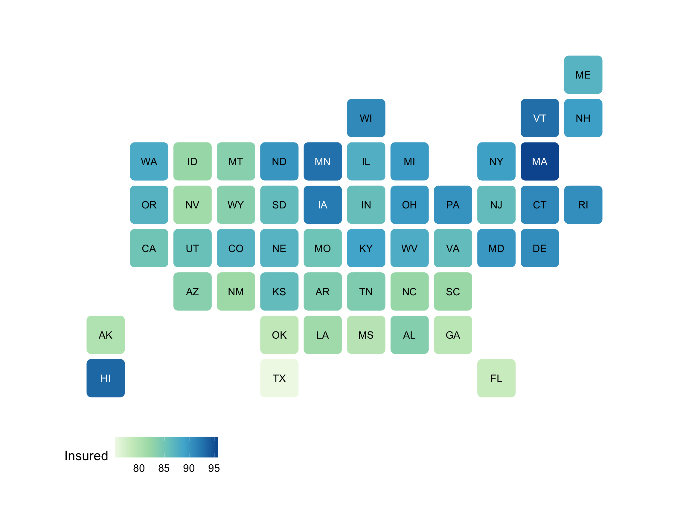
Hexbin Maps

library(statebins)
statebins(state_data = USStates,
          state_col = "State",
          value_col = "Insured",
          ggplot2_scale_function =
            ggplot2::scale_fill_distiller,
          direction = 1, type = "seq", palette = 4,
          round = TRUE) +
  theme_statebins()

New data: volcano eruptions

Eruptions <- read_csv("data/GVP_Eruption_Results.csv")
select(Eruptions, VolcanoName, StartYear, Latitude, Longitude) %>%
  glimpse()
Rows: 11,019
Columns: 4
$ VolcanoName <chr> "Bulusan", "Alaid", "Turrialba", "San Miguel", "Chill\xe0n…
$ StartYear   <dbl> 2016, 2016, 2016, 2016, 2016, 2016, 2015, 2015, 2015, 2015…
$ Latitude    <dbl> 12.770, 50.861, 10.025, 13.434, -36.863, 1.112, 11.984, 37…
$ Longitude   <dbl> 124.050, 155.565, -83.767, -88.269, -71.377, 124.737, -86.…
library(rnaturalearth)
world <- rnaturalearth::countries110
world
Simple feature collection with 177 features and 168 fields
Geometry type: MULTIPOLYGON
Dimension:     XY
Bounding box:  xmin: -180 ymin: -90 xmax: 180 ymax: 83.64513
Geodetic CRS:  WGS 84
First 10 features:
        featurecla scalerank LABELRANK                  SOVEREIGNT SOV_A3
1  Admin-0 country         1         6                        Fiji    FJI
2  Admin-0 country         1         3 United Republic of Tanzania    TZA
3  Admin-0 country         1         7              Western Sahara    SAH
4  Admin-0 country         1         2                      Canada    CAN
5  Admin-0 country         1         2    United States of America    US1
6  Admin-0 country         1         3                  Kazakhstan    KA1
7  Admin-0 country         1         3                  Uzbekistan    UZB
8  Admin-0 country         1         2            Papua New Guinea    PNG
9  Admin-0 country         1         2                   Indonesia    IDN
10 Admin-0 country         1         2                   Argentina    ARG
   ADM0_DIF LEVEL              TYPE TLC                       ADMIN ADM0_A3
1         0     2 Sovereign country   1                        Fiji     FJI
2         0     2 Sovereign country   1 United Republic of Tanzania     TZA
3         0     2     Indeterminate   1              Western Sahara     SAH
4         0     2 Sovereign country   1                      Canada     CAN
5         1     2           Country   1    United States of America     USA
6         1     1       Sovereignty   1                  Kazakhstan     KAZ
7         0     2 Sovereign country   1                  Uzbekistan     UZB
8         0     2 Sovereign country   1            Papua New Guinea     PNG
9         0     2 Sovereign country   1                   Indonesia     IDN
10        0     2 Sovereign country   1                   Argentina     ARG
   GEOU_DIF                  GEOUNIT GU_A3 SU_DIF          SUBUNIT SU_A3
1         0                     Fiji   FJI      0             Fiji   FJI
2         0                 Tanzania   TZA      0         Tanzania   TZA
3         0           Western Sahara   SAH      0   Western Sahara   SAH
4         0                   Canada   CAN      0           Canada   CAN
5         0 United States of America   USA      0    United States   USA
6         0               Kazakhstan   KAZ      0       Kazakhstan   KAZ
7         0               Uzbekistan   UZB      0       Uzbekistan   UZB
8         0         Papua New Guinea   PNG      1 Papua New Guinea   PN1
9         0                Indonesia   IDN      0        Indonesia   IDN
10        0                Argentina   ARG      0        Argentina   ARG
   BRK_DIFF                     NAME        NAME_LONG BRK_A3         BRK_NAME
1         0                     Fiji             Fiji    FJI             Fiji
2         0                 Tanzania         Tanzania    TZA         Tanzania
3         1                W. Sahara   Western Sahara    B28        W. Sahara
4         0                   Canada           Canada    CAN           Canada
5         0 United States of America    United States    USA    United States
6         0               Kazakhstan       Kazakhstan    KAZ       Kazakhstan
7         0               Uzbekistan       Uzbekistan    UZB       Uzbekistan
8         0         Papua New Guinea Papua New Guinea    PN1 Papua New Guinea
9         0                Indonesia        Indonesia    IDN        Indonesia
10        0                Argentina        Argentina    ARG        Argentina
   BRK_GROUP  ABBREV POSTAL                             FORMAL_EN FORMAL_FR
1       <NA>    Fiji     FJ                      Republic of Fiji      <NA>
2       <NA>   Tanz.     TZ           United Republic of Tanzania      <NA>
3       <NA> W. Sah.     WS      Sahrawi Arab Democratic Republic      <NA>
4       <NA>    Can.     CA                                Canada      <NA>
5       <NA>  U.S.A.     US              United States of America      <NA>
6       <NA>    Kaz.     KZ                Republic of Kazakhstan      <NA>
7       <NA>    Uzb.     UZ                Republic of Uzbekistan      <NA>
8       <NA>  P.N.G.     PG Independent State of Papua New Guinea      <NA>
9       <NA>   Indo.   INDO                 Republic of Indonesia      <NA>
10      <NA>    Arg.     AR                    Argentine Republic      <NA>
         NAME_CIAWF NOTE_ADM0                        NOTE_BRK
1              Fiji      <NA>                            <NA>
2          Tanzania      <NA>                            <NA>
3    Western Sahara      <NA> Self admin.; Claimed by Morocco
4            Canada      <NA>                            <NA>
5     United States      <NA>                            <NA>
6        Kazakhstan      <NA>                            <NA>
7        Uzbekistan      <NA>                            <NA>
8  Papua New Guinea      <NA>                            <NA>
9         Indonesia      <NA>                            <NA>
10        Argentina      <NA>                            <NA>
                  NAME_SORT NAME_ALT MAPCOLOR7 MAPCOLOR8 MAPCOLOR9 MAPCOLOR13
1                      Fiji     <NA>         5         1         2          2
2                  Tanzania     <NA>         3         6         2          2
3            Western Sahara     <NA>         4         7         4          4
4                    Canada     <NA>         6         6         2          2
5  United States of America     <NA>         4         5         1          1
6                Kazakhstan     <NA>         6         1         6          1
7                Uzbekistan     <NA>         2         3         5          4
8          Papua New Guinea     <NA>         4         2         3          1
9                 Indonesia     <NA>         6         6         6         11
10                Argentina     <NA>         3         1         3         13
     POP_EST POP_RANK POP_YEAR   GDP_MD GDP_YEAR                   ECONOMY
1     889953       11     2019     5496     2019      6. Developing region
2   58005463       16     2019    63177     2019 7. Least developed region
3     603253       11     2017      907     2007 7. Least developed region
4   37589262       15     2019  1736425     2019   1. Developed region: G7
5  328239523       17     2019 21433226     2019   1. Developed region: G7
6   18513930       14     2019   181665     2019      6. Developing region
7   33580650       15     2019    57921     2019      6. Developing region
8    8776109       13     2019    24829     2019      6. Developing region
9  270625568       17     2019  1119190     2019  4. Emerging region: MIKT
10  44938712       15     2019   445445     2019   5. Emerging region: G20
               INCOME_GRP FIPS_10 ISO_A2 ISO_A2_EH ISO_A3 ISO_A3_EH ISO_N3
1  4. Lower middle income      FJ     FJ        FJ    FJI       FJI    242
2           5. Low income      TZ     TZ        TZ    TZA       TZA    834
3           5. Low income      WI     EH        EH    ESH       ESH    732
4    1. High income: OECD      CA     CA        CA    CAN       CAN    124
5    1. High income: OECD      US     US        US    USA       USA    840
6  3. Upper middle income      KZ     KZ        KZ    KAZ       KAZ    398
7  4. Lower middle income      UZ     UZ        UZ    UZB       UZB    860
8  4. Lower middle income      PP     PG        PG    PNG       PNG    598
9  4. Lower middle income      ID     ID        ID    IDN       IDN    360
10 3. Upper middle income      AR     AR        AR    ARG       ARG    032
   ISO_N3_EH UN_A3 WB_A2 WB_A3   WOE_ID WOE_ID_EH
1        242   242    FJ   FJI 23424813  23424813
2        834   834    TZ   TZA 23424973  23424973
3        732   732   -99   -99 23424990  23424990
4        124   124    CA   CAN 23424775  23424775
5        840   840    US   USA 23424977  23424977
6        398   398    KZ   KAZ      -90  23424871
7        860   860    UZ   UZB 23424980  23424980
8        598   598    PG   PNG 23424926  23424926
9        360   360    ID   IDN 23424846  23424846
10       032   032    AR   ARG 23424747  23424747
                                                      WOE_NOTE ADM0_ISO
1                                   Exact WOE match as country      FJI
2                                   Exact WOE match as country      TZA
3                                   Exact WOE match as country      B28
4                                   Exact WOE match as country      CAN
5                                   Exact WOE match as country      USA
6  Includes Baykonur Cosmodrome as an Admin-1 states provinces      KAZ
7                                   Exact WOE match as country      UZB
8                                   Exact WOE match as country      PN1
9                                   Exact WOE match as country      IDN
10                                  Exact WOE match as country      ARG
   ADM0_DIFF ADM0_TLC ADM0_A3_US ADM0_A3_FR ADM0_A3_RU ADM0_A3_ES ADM0_A3_CN
1       <NA>      FJI        FJI        FJI        FJI        FJI        FJI
2       <NA>      TZA        TZA        TZA        TZA        TZA        TZA
3       <NA>      B28        SAH        MAR        SAH        SAH        SAH
4       <NA>      CAN        CAN        CAN        CAN        CAN        CAN
5       <NA>      USA        USA        USA        USA        USA        USA
6       <NA>      KAZ        KAZ        KAZ        KAZ        KAZ        KAZ
7       <NA>      UZB        UZB        UZB        UZB        UZB        UZB
8       <NA>      PN1        PNG        PNG        PNG        PNG        PNG
9       <NA>      IDN        IDN        IDN        IDN        IDN        IDN
10      <NA>      ARG        ARG        ARG        ARG        ARG        ARG
   ADM0_A3_TW ADM0_A3_IN ADM0_A3_NP ADM0_A3_PK ADM0_A3_DE ADM0_A3_GB ADM0_A3_BR
1         FJI        FJI        FJI        FJI        FJI        FJI        FJI
2         TZA        TZA        TZA        TZA        TZA        TZA        TZA
3         SAH        MAR        SAH        SAH        SAH        SAH        SAH
4         CAN        CAN        CAN        CAN        CAN        CAN        CAN
5         USA        USA        USA        USA        USA        USA        USA
6         KAZ        KAZ        KAZ        KAZ        KAZ        KAZ        KAZ
7         UZB        UZB        UZB        UZB        UZB        UZB        UZB
8         PNG        PNG        PNG        PNG        PNG        PNG        PNG
9         IDN        IDN        IDN        IDN        IDN        IDN        IDN
10        ARG        ARG        ARG        ARG        ARG        ARG        ARG
   ADM0_A3_IL ADM0_A3_PS ADM0_A3_SA ADM0_A3_EG ADM0_A3_MA ADM0_A3_PT ADM0_A3_AR
1         FJI        FJI        FJI        FJI        FJI        FJI        FJI
2         TZA        TZA        TZA        TZA        TZA        TZA        TZA
3         SAH        MAR        MAR        SAH        MAR        SAH        SAH
4         CAN        CAN        CAN        CAN        CAN        CAN        CAN
5         USA        USA        USA        USA        USA        USA        USA
6         KAZ        KAZ        KAZ        KAZ        KAZ        KAZ        KAZ
7         UZB        UZB        UZB        UZB        UZB        UZB        UZB
8         PNG        PNG        PNG        PNG        PNG        PNG        PNG
9         IDN        IDN        IDN        IDN        IDN        IDN        IDN
10        ARG        ARG        ARG        ARG        ARG        ARG        ARG
   ADM0_A3_JP ADM0_A3_KO ADM0_A3_VN ADM0_A3_TR ADM0_A3_ID ADM0_A3_PL ADM0_A3_GR
1         FJI        FJI        FJI        FJI        FJI        FJI        FJI
2         TZA        TZA        TZA        TZA        TZA        TZA        TZA
3         SAH        SAH        SAH        MAR        MAR        MAR        SAH
4         CAN        CAN        CAN        CAN        CAN        CAN        CAN
5         USA        USA        USA        USA        USA        USA        USA
6         KAZ        KAZ        KAZ        KAZ        KAZ        KAZ        KAZ
7         UZB        UZB        UZB        UZB        UZB        UZB        UZB
8         PNG        PNG        PNG        PNG        PNG        PNG        PNG
9         IDN        IDN        IDN        IDN        IDN        IDN        IDN
10        ARG        ARG        ARG        ARG        ARG        ARG        ARG
   ADM0_A3_IT ADM0_A3_NL ADM0_A3_SE ADM0_A3_BD ADM0_A3_UA ADM0_A3_UN ADM0_A3_WB
1         FJI        FJI        FJI        FJI        FJI        -99        -99
2         TZA        TZA        TZA        TZA        TZA        -99        -99
3         SAH        MAR        SAH        SAH        SAH        -99        -99
4         CAN        CAN        CAN        CAN        CAN        -99        -99
5         USA        USA        USA        USA        USA        -99        -99
6         KAZ        KAZ        KAZ        KAZ        KAZ        -99        -99
7         UZB        UZB        UZB        UZB        UZB        -99        -99
8         PNG        PNG        PNG        PNG        PNG        -99        -99
9         IDN        IDN        IDN        IDN        IDN        -99        -99
10        ARG        ARG        ARG        ARG        ARG        -99        -99
       CONTINENT REGION_UN          SUBREGION                  REGION_WB
1        Oceania   Oceania          Melanesia        East Asia & Pacific
2         Africa    Africa     Eastern Africa         Sub-Saharan Africa
3         Africa    Africa    Northern Africa Middle East & North Africa
4  North America  Americas   Northern America              North America
5  North America  Americas   Northern America              North America
6           Asia      Asia       Central Asia      Europe & Central Asia
7           Asia      Asia       Central Asia      Europe & Central Asia
8        Oceania   Oceania          Melanesia        East Asia & Pacific
9           Asia      Asia South-Eastern Asia        East Asia & Pacific
10 South America  Americas      South America  Latin America & Caribbean
   NAME_LEN LONG_LEN ABBREV_LEN TINY HOMEPART MIN_ZOOM MIN_LABEL MAX_LABEL
1         4        4          4  -99        1      0.0       3.0       8.0
2         8        8          5  -99        1      0.0       3.0       8.0
3         9       14          7  -99        1      4.7       6.0      11.0
4         6        6          4  -99        1      0.0       1.7       5.7
5        24       13          6  -99        1      0.0       1.7       5.7
6        10       10          4  -99        1      0.0       2.7       7.0
7        10       10          4    5        1      0.0       3.0       8.0
8        16       16          6  -99        1      0.0       2.5       7.5
9         9        9          5  -99        1      0.0       1.7       6.7
10        9        9          4  -99        1      0.0       2.0       7.0
      LABEL_X    LABEL_Y      NE_ID WIKIDATAID             NAME_AR
1   177.97543 -17.826099 1159320625       Q712                فيجي
2    34.95918  -6.051866 1159321337       Q924             تنزانيا
3   -12.63030  23.967592 1159321223      Q6250     الصحراء الغربية
4  -101.91070  60.324287 1159320467        Q16                كندا
5   -97.48260  39.538479 1159321369        Q30    الولايات المتحدة
6    68.68555  49.054149 1159320967       Q232           كازاخستان
7    64.00543  41.693603 1159321405       Q265           أوزبكستان
8   143.91022  -5.695285 1159321173       Q691 بابوا غينيا الجديدة
9   101.89295  -0.954404 1159320845       Q252           إندونيسيا
10  -64.17333 -33.501159 1159320331       Q414           الأرجنتين
           NAME_BN            NAME_DE                  NAME_EN
1             ফিজি            Fidschi                     Fiji
2        তানজানিয়া           Tansania                 Tanzania
3     পশ্চিম সাহারা         Westsahara           Western Sahara
4           কানাডা             Kanada                   Canada
5  মার্কিন যুক্তরাষ্ট্র Vereinigte Staaten United States of America
6        কাজাখস্তান         Kasachstan               Kazakhstan
7       উজবেকিস্তান         Usbekistan               Uzbekistan
8    পাপুয়া নিউগিনি    Papua-Neuguinea         Papua New Guinea
9       ইন্দোনেশিয়া         Indonesien                Indonesia
10       আর্জেন্টিনা        Argentinien                Argentina
              NAME_ES             NAME_FA                   NAME_FR
1                Fiyi                فیجی                     Fidji
2            Tanzania            تانزانیا                  Tanzanie
3   Sahara Occidental          صحرای غربی         Sahara occidental
4              Canadá              کانادا                    Canada
5      Estados Unidos ایالات متحده آمریکا                États-Unis
6          Kazajistán            قزاقستان                Kazakhstan
7          Uzbekistán            ازبکستان               Ouzbékistan
8  Papúa Nueva Guinea       پاپوآ گینه نو Papouasie-Nouvelle-Guinée
9           Indonesia             اندونزی                 Indonésie
10          Argentina            آرژانتین                 Argentine
                       NAME_EL           NAME_HE          NAME_HI
1                        Φίτζι             פיג'י             फ़िजी
2                     Τανζανία            טנזניה          तंज़ानिया
3                Δυτική Σαχάρα      סהרה המערבית     पश्चिमी सहारा
4                      Καναδάς              קנדה            कनाडा
5  Ηνωμένες Πολιτείες Αμερικής       ארצות הברית संयुक्त राज्य अमेरिका
6                    Καζακστάν            קזחסטן        कज़ाख़िस्तान
7                 Ουζμπεκιστάν         אוזבקיסטן        उज़्बेकिस्तान
8           Παπούα Νέα Γουινέα פפואה גינאה החדשה     पापुआ न्यू गिनी
9                    Ινδονησία         אינדונזיה         इंडोनेशिया
10                   Αργεντινή          ארגנטינה         अर्जेण्टीना
                     NAME_HU         NAME_ID               NAME_IT
1            Fidzsi-szigetek            Fiji                  Figi
2                   Tanzánia        Tanzania              Tanzania
3             Nyugat-Szahara    Sahara Barat    Sahara Occidentale
4                     Kanada          Kanada                Canada
5  Amerikai Egyesült Államok Amerika Serikat Stati Uniti d'America
6                 Kazahsztán      Kazakhstan            Kazakistan
7                Üzbegisztán      Uzbekistan            Uzbekistan
8            Pápua Új-Guinea    Papua Nugini    Papua Nuova Guinea
9                  Indonézia       Indonesia             Indonesia
10                 Argentína       Argentina             Argentina
              NAME_JA      NAME_KO                      NAME_NL
1            フィジー         피지                         Fiji
2          タンザニア     탄자니아                     Tanzania
3            西サハラ     서사하라            Westelijke Sahara
4              カナダ       캐나다                       Canada
5      アメリカ合衆国         미국 Verenigde Staten van Amerika
6        カザフスタン   카자흐스탄                   Kazachstan
7      ウズベキスタン 우즈베키스탄                  Oezbekistan
8  パプアニューギニア 파푸아뉴기니          Papoea-Nieuw-Guinea
9        インドネシア   인도네시아                    Indonesië
10       アルゼンチン   아르헨티나                   Argentinië
             NAME_PL          NAME_PT              NAME_RU          NAME_SV
1              Fidżi             Fiji                Фиджи             Fiji
2           Tanzania         Tanzânia             Танзания         Tanzania
3   Sahara Zachodnia   Sara Ocidental      Западная Сахара       Västsahara
4             Kanada           Canadá               Канада           Kanada
5  Stany Zjednoczone   Estados Unidos                  США              USA
6         Kazachstan      Cazaquistão            Казахстан        Kazakstan
7         Uzbekistan      Uzbequistão           Узбекистан       Uzbekistan
8  Papua-Nowa Gwinea Papua-Nova Guiné Папуа — Новая Гвинея Papua Nya Guinea
9          Indonezja        Indonésia            Индонезия       Indonesien
10         Argentyna        Argentina            Аргентина        Argentina
                       NAME_TR                 NAME_UK                NAME_UR
1                         Fiji                   Фіджі                    فجی
2                     Tanzanya                Танзанія                تنزانیہ
3                   Batı Sahra          Західна Сахара            مغربی صحارا
4                       Kanada                  Канада                 کینیڈا
5  Amerika Birleşik Devletleri Сполучені Штати Америки ریاستہائے متحدہ امریکا
6                   Kazakistan               Казахстан               قازقستان
7                   Özbekistan              Узбекистан               ازبکستان
8              Papua Yeni Gine       Папуа Нова Гвінея          پاپوا نیو گنی
9                    Endonezya               Індонезія              انڈونیشیا
10                    Arjantin               Аргентина               ارجنٹائن
            NAME_VI        NAME_ZH       NAME_ZHT         FCLASS_ISO TLC_DIFF
1              Fiji           斐济           斐濟    Admin-0 country     <NA>
2          Tanzania       坦桑尼亚       坦尚尼亞    Admin-0 country     <NA>
3        Tây Sahara       西撒哈拉       西撒哈拉 Admin-0 dependency     <NA>
4            Canada         加拿大         加拿大    Admin-0 country     <NA>
5            Hoa Kỳ           美国           美國    Admin-0 country     <NA>
6        Kazakhstan     哈萨克斯坦         哈薩克    Admin-0 country     <NA>
7        Uzbekistan   乌兹别克斯坦       烏茲別克    Admin-0 country     <NA>
8  Papua New Guinea 巴布亚新几内亚 巴布亞紐幾內亞    Admin-0 country     <NA>
9         Indonesia     印度尼西亚     印度尼西亞    Admin-0 country     <NA>
10        Argentina         阿根廷         阿根廷    Admin-0 country     <NA>
           FCLASS_TLC FCLASS_US    FCLASS_FR FCLASS_RU FCLASS_ES FCLASS_CN
1     Admin-0 country      <NA>         <NA>      <NA>      <NA>      <NA>
2     Admin-0 country      <NA>         <NA>      <NA>      <NA>      <NA>
3  Admin-0 dependency      <NA> Unrecognized      <NA>      <NA>      <NA>
4     Admin-0 country      <NA>         <NA>      <NA>      <NA>      <NA>
5     Admin-0 country      <NA>         <NA>      <NA>      <NA>      <NA>
6     Admin-0 country      <NA>         <NA>      <NA>      <NA>      <NA>
7     Admin-0 country      <NA>         <NA>      <NA>      <NA>      <NA>
8     Admin-0 country      <NA>         <NA>      <NA>      <NA>      <NA>
9     Admin-0 country      <NA>         <NA>      <NA>      <NA>      <NA>
10    Admin-0 country      <NA>         <NA>      <NA>      <NA>      <NA>
   FCLASS_TW    FCLASS_IN FCLASS_NP FCLASS_PK FCLASS_DE FCLASS_GB FCLASS_BR
1       <NA>         <NA>      <NA>      <NA>      <NA>      <NA>      <NA>
2       <NA>         <NA>      <NA>      <NA>      <NA>      <NA>      <NA>
3       <NA> Unrecognized      <NA>      <NA>      <NA>      <NA>      <NA>
4       <NA>         <NA>      <NA>      <NA>      <NA>      <NA>      <NA>
5       <NA>         <NA>      <NA>      <NA>      <NA>      <NA>      <NA>
6       <NA>         <NA>      <NA>      <NA>      <NA>      <NA>      <NA>
7       <NA>         <NA>      <NA>      <NA>      <NA>      <NA>      <NA>
8       <NA>         <NA>      <NA>      <NA>      <NA>      <NA>      <NA>
9       <NA>         <NA>      <NA>      <NA>      <NA>      <NA>      <NA>
10      <NA>         <NA>      <NA>      <NA>      <NA>      <NA>      <NA>
   FCLASS_IL    FCLASS_PS    FCLASS_SA FCLASS_EG    FCLASS_MA FCLASS_PT
1       <NA>         <NA>         <NA>      <NA>         <NA>      <NA>
2       <NA>         <NA>         <NA>      <NA>         <NA>      <NA>
3       <NA> Unrecognized Unrecognized      <NA> Unrecognized      <NA>
4       <NA>         <NA>         <NA>      <NA>         <NA>      <NA>
5       <NA>         <NA>         <NA>      <NA>         <NA>      <NA>
6       <NA>         <NA>         <NA>      <NA>         <NA>      <NA>
7       <NA>         <NA>         <NA>      <NA>         <NA>      <NA>
8       <NA>         <NA>         <NA>      <NA>         <NA>      <NA>
9       <NA>         <NA>         <NA>      <NA>         <NA>      <NA>
10      <NA>         <NA>         <NA>      <NA>         <NA>      <NA>
   FCLASS_AR FCLASS_JP FCLASS_KO FCLASS_VN    FCLASS_TR    FCLASS_ID
1       <NA>      <NA>      <NA>      <NA>         <NA>         <NA>
2       <NA>      <NA>      <NA>      <NA>         <NA>         <NA>
3       <NA>      <NA>      <NA>      <NA> Unrecognized Unrecognized
4       <NA>      <NA>      <NA>      <NA>         <NA>         <NA>
5       <NA>      <NA>      <NA>      <NA>         <NA>         <NA>
6       <NA>      <NA>      <NA>      <NA>         <NA>         <NA>
7       <NA>      <NA>      <NA>      <NA>         <NA>         <NA>
8       <NA>      <NA>      <NA>      <NA>         <NA>         <NA>
9       <NA>      <NA>      <NA>      <NA>         <NA>         <NA>
10      <NA>      <NA>      <NA>      <NA>         <NA>         <NA>
      FCLASS_PL FCLASS_GR FCLASS_IT    FCLASS_NL FCLASS_SE FCLASS_BD FCLASS_UA
1          <NA>      <NA>      <NA>         <NA>      <NA>      <NA>      <NA>
2          <NA>      <NA>      <NA>         <NA>      <NA>      <NA>      <NA>
3  Unrecognized      <NA>      <NA> Unrecognized      <NA>      <NA>      <NA>
4          <NA>      <NA>      <NA>         <NA>      <NA>      <NA>      <NA>
5          <NA>      <NA>      <NA>         <NA>      <NA>      <NA>      <NA>
6          <NA>      <NA>      <NA>         <NA>      <NA>      <NA>      <NA>
7          <NA>      <NA>      <NA>         <NA>      <NA>      <NA>      <NA>
8          <NA>      <NA>      <NA>         <NA>      <NA>      <NA>      <NA>
9          <NA>      <NA>      <NA>         <NA>      <NA>      <NA>      <NA>
10         <NA>      <NA>      <NA>         <NA>      <NA>      <NA>      <NA>
                         geometry
1  MULTIPOLYGON (((180 -16.067...
2  MULTIPOLYGON (((33.90371 -0...
3  MULTIPOLYGON (((-8.66559 27...
4  MULTIPOLYGON (((-122.84 49,...
5  MULTIPOLYGON (((-122.84 49,...
6  MULTIPOLYGON (((87.35997 49...
7  MULTIPOLYGON (((55.96819 41...
8  MULTIPOLYGON (((141.0002 -2...
9  MULTIPOLYGON (((141.0002 -2...
10 MULTIPOLYGON (((-68.63401 -...

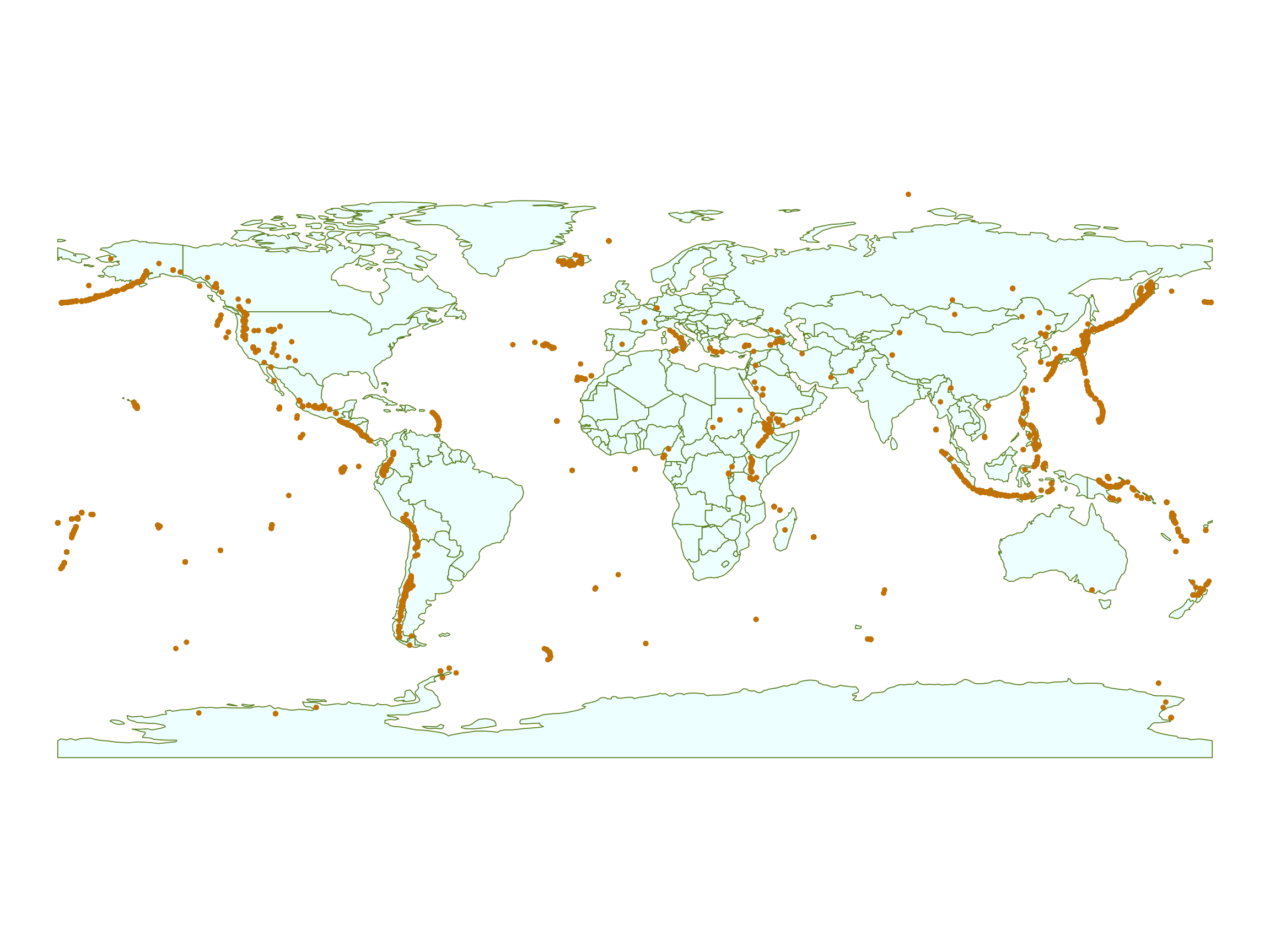
Static Maps

Eruptions_sf <- Eruptions %>%
  st_as_sf(coords = c("Longitude",
                      "Latitude"),
           crs = "EPSG:4269")

ggplot(data = world) +
  geom_sf(fill = "azure",
          color = "olivedrab4") +
  geom_sf(data = Eruptions_sf,
          color = "orange3",
          size = 0.5) +
  theme_void()

  • What if we want to zoom in?

Alluetian Islands
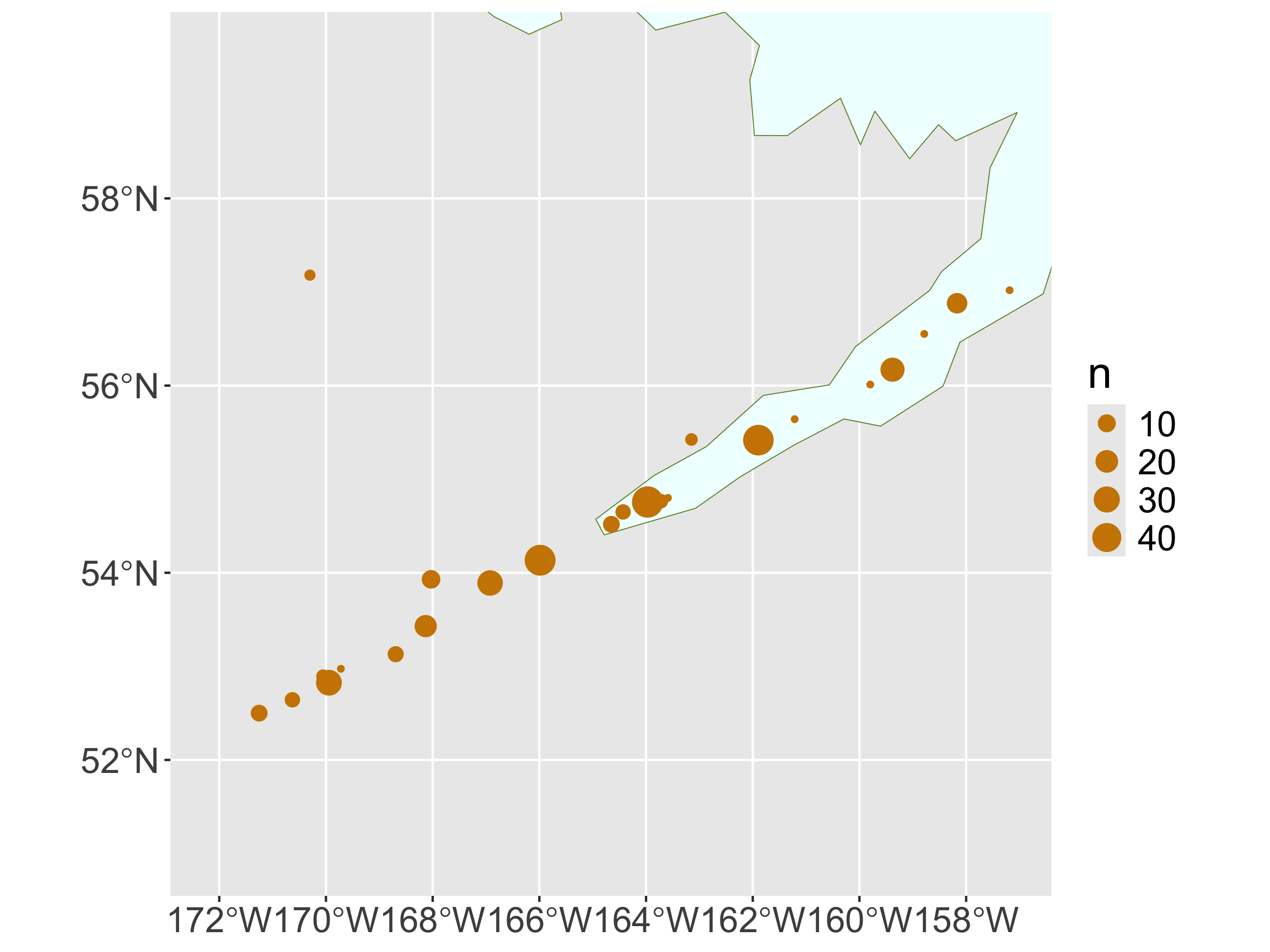
eruption_count <- count(Eruptions,
                        VolcanoName, 
                        Latitude,
                        Longitude) %>%
  filter(Longitude > -172.164,
         Longitude < -157.1507,
         Latitude > 50.977,
         Latitude < 59.5617) %>%
  arrange(desc(n)) %>%
  st_as_sf(coords = c("Longitude",
                      "Latitude"),
           crs = "EPSG:4269")
eruption_count
Simple feature collection with 24 features and 2 fields
Geometry type: POINT
Dimension:     XY
Bounding box:  xmin: -171.252 ymin: 52.5 xmax: -157.185 ymax: 57.18
Geodetic CRS:  NAD83
# A tibble: 24 × 3
   VolcanoName     n          geometry
 * <chr>       <int>       <POINT [°]>
 1 Shishaldin     49  (-163.97 54.756)
 2 Akutan         47 (-165.986 54.134)
 3 Pavlof         46 (-161.894 55.417)
 4 Cleveland      29 (-169.944 52.825)
 5 Makushin       28 (-166.923 53.891)
 6 Veniaminof     24   (-159.38 56.17)
 7 Okmok          19   (-168.13 53.43)
 8 Aniakchak      15   (-158.17 56.88)
 9 Bogoslof       11   (-168.03 53.93)
10 Amukta          8   (-171.252 52.5)
# ℹ 14 more rows

Alluetian Islands

ggplot() +
  geom_sf(data = world, 
          fill = "azure",
          color = "olivedrab4") +
  geom_sf(data = eruption_count,
          mapping = aes(size = n),
          color = "orange3") +
  coord_sf(xlim = c(-172.164, -157.1507),
           ylim = c(50.977, 59.5617))

  • Not a great base layer…
  • What about dynamic zooming and clickable labels?

Interactive Maps with leaflet

  • Syntax similar to ggplot2 and dplyr
  • Interactive zooming
  • Embed interactive map into Quarto documents (HTML output)
  • Can take lat/lon or geometry/sf objects

Interactive Maps with leaflet

library(leaflet)
leaflet() %>%
  addTiles() %>%
  addCircleMarkers(data = eruption_count,
                   radius = ~sqrt(n), 
                   stroke = FALSE,
                   fillOpacity = 0.9,
                   color = "orange")
  • First Layer: leaflet()
    • Creates the map widget
  • Second layer: addTiles()
  • Additional layers: addMarkers(), addPolygons()

Interactive Maps with leaflet

library(leaflet)
leaflet() %>%
  addTiles() %>%
  addCircleMarkers(data = eruption_count,
                   radius = ~sqrt(n), 
                   stroke = FALSE,
                   fillOpacity = 0.9)

Clusters

leaflet() %>%
  setView(lng = -160, lat = 55, zoom = 6) %>%
  addTiles() %>%
  addCircleMarkers(data = eruption_count, 
                   clusterOptions =
                     markerClusterOptions())

Zooming Constraints

leaflet(options = 
          leafletOptions(minZoom = 3,
                         maxZoom = 7)) %>%
  addTiles() %>%
  addCircleMarkers(data = eruption_count,
                   radius = ~sqrt(n))

Other Markers

leaflet() %>% 
  setView(lng = -160, lat = 55, zoom = 4) %>%
  addTiles() %>%
  addMarkers(data = eruption_count, 
             label = ~as.character(n))

Custom Icons

volcano  <- makeIcon(
  iconUrl = "https://raw.githubusercontent.com/Reed-Data-Science/Reed-Data-Science.github.io/refs/heads/main/slides/img/volcano.png",
  iconWidth = 20, iconHeight = 20)
volcano
$iconUrl
[1] "https://raw.githubusercontent.com/Reed-Data-Science/Reed-Data-Science.github.io/refs/heads/main/slides/img/volcano.png"

$iconWidth
[1] 20

$iconHeight
[1] 20

attr(,"class")
[1] "leaflet_icon"

Custom Icons

leaflet() %>% 
  setView(lng = -160, lat = 55, zoom = 4) %>%
  addTiles() %>%
  addMarkers(data = eruption_count, 
             label = ~as.character(n),
             icon = volcano)

Pop-Ups

content <- paste("<b>",
                 eruption_count$VolcanoName, 
                 "</b></br>",
                 "Number of eruptions:",
                 eruption_count$n)
content
 [1] "<b> Shishaldin </b></br> Number of eruptions: 49"    
 [2] "<b> Akutan </b></br> Number of eruptions: 47"        
 [3] "<b> Pavlof </b></br> Number of eruptions: 46"        
 [4] "<b> Cleveland </b></br> Number of eruptions: 29"     
 [5] "<b> Makushin </b></br> Number of eruptions: 28"      
 [6] "<b> Veniaminof </b></br> Number of eruptions: 24"    
 [7] "<b> Okmok </b></br> Number of eruptions: 19"         
 [8] "<b> Aniakchak </b></br> Number of eruptions: 15"     
 [9] "<b> Bogoslof </b></br> Number of eruptions: 11"      
[10] "<b> Amukta </b></br> Number of eruptions: 8"         
[11] "<b> Westdahl </b></br> Number of eruptions: 8"       
[12] "<b> Vsevidof </b></br> Number of eruptions: 7"       
[13] "<b> Fisher </b></br> Number of eruptions: 6"         
[14] "<b> Yunaska </b></br> Number of eruptions: 6"        
[15] "<b> Isanotski </b></br> Number of eruptions: 5"      
[16] "<b> Carlisle </b></br> Number of eruptions: 4"       
[17] "<b> Amak </b></br> Number of eruptions: 3"           
[18] "<b> St. Paul Island </b></br> Number of eruptions: 2"
[19] "<b> Black Peak </b></br> Number of eruptions: 1"     
[20] "<b> Dana </b></br> Number of eruptions: 1"           
[21] "<b> Kagamil </b></br> Number of eruptions: 1"        
[22] "<b> Kupreanof </b></br> Number of eruptions: 1"      
[23] "<b> Roundtop </b></br> Number of eruptions: 1"       
[24] "<b> Yantarni </b></br> Number of eruptions: 1"       

Pop-Ups

leaflet() %>% 
  setView(lng = -160, lat = 55, zoom = 4) %>%
  addTiles() %>%
  addMarkers(data = eruption_count, 
             popup = content,
             icon = volcano)

Other Tiles

library(leaflet.extras)
leaflet() %>% 
  setView(lng = -122.6308,
          lat = 45.4811,
          zoom = 15) %>%     
  addProviderTiles(providers$Stadia.StamenWatercolor)

Other Tiles

leaflet() %>% 
  setView(lng = -122.6308,
          lat = 45.4811,
          zoom = 15) %>%     
 addProviderTiles(
   providers$Stadia.StamenTerrain) %>%
  addMiniMap()

Other Tiles

leaflet() %>% 
  setView(lng = -122.6308,
          lat = 45.4811,
          zoom = 3) %>%     
  addProviderTiles(
    "NASAGIBS.ViirsEarthAtNight2012") 

Interactive Choropleth Map

pal <- colorNumeric(palette = "GnBu",
                    domain = wa$estimate,
                    reverse = FALSE)
pal(wa$estimate)
 [1] "#5CB9CF" "#77CAC6" "#CDEBC6" "#D2EECC" "#A1DAB8" "#90D3BD" "#45A8CD"
 [8] "#56B6D1" "#AADEB6" "#4CB1D2" "#F7FCF0" "#F2FAEC" "#D1EDCB" "#E3F4DE"
[15] "#CDEBC6" "#AADEB6" "#C8E9C3" "#87D0C1" "#C8E9C3" "#DEF2D9" "#084081"
[22] "#227FB7" "#DBF1D6" "#7CCCC4" "#C1E7C0" "#C4E8C1" "#D1EDCB" "#95D5BC"
[29] "#9ED9B9" "#CBEBC5" "#ECF8E6" "#DEF2D9" "#CFECC8" "#DBF1D5" "#D8F0D2"
[36] "#BEE6BF" "#C7E9C3" "#C8EAC3" "#70C4C9"

Interactive Choropleth Map

wa %>%
  leaflet() %>%
  addTiles() %>%
  addPolygons(popup = ~NAME,
              color = ~pal(estimate),
              stroke = FALSE,
              fillOpacity = 0.9) 
Warning: sf layer has inconsistent datum (+proj=longlat +datum=NAD83 +no_defs).
Need '+proj=longlat +datum=WGS84'
  • Throws a warning about the projection

Interactive Choropleth Map

wa %>%
  sf::st_transform(crs = "EPSG:4326") %>%    
  leaflet() %>%
  addTiles() %>%
  addPolygons(popup = ~NAME,
              color = ~pal(estimate),
              stroke = FALSE,
              fillOpacity = 0.9) 

Interactive Choropleth Map

wa %>%
  sf::st_transform(crs = "EPSG:4326") %>%  
  leaflet() %>%
  addTiles() %>%
  addPolygons(popup = ~NAME,
              color = ~pal(estimate),
              stroke = FALSE,
              fillOpacity = 0.9) %>%
  addLegend("bottomright", pal = pal, 
            values = ~estimate,
            title = "Median Income",
            opacity = 1)

Next week

  • More spatial data:
    • Spatial computations
    • Raster data
  • Learn to develop shiny dashboards
    • for increased user interactivity!
    • (and for Project 1)

Resources for learning more about spatial data